Exercises

Outcome regression

For these exercises, assume the measured-confounding SCM with covariates \(X\), exposure \(A\), and outcome \(Y\). Assume observations related to different units are i.i.d. and the relevant conditional means are defined. You may use a calculator. Keep additional digits during calculations and report your final answers to two decimal places.

1. Estimating means from counts

Both \(X\) and \(A\) are binary, and \(Y\) indicates an adverse outcome. The dataset has the following counts:

\(X\)	\(A\)	Number of people	Number with \(Y=1\)
0	0	30	12
0	1	10	2
1	0	20	12
1	1	40	16

1. Estimate \(\mu(X,A)\) for all four combinations of \(X\) and \(A\).

2. Find \(\hat\mu(X,1)\) and \(\hat\mu(X,0)\) for someone whose recorded values are \(X=1,A=0\).

3. Estimate \(E\left[Y(1)\right]\) and \(E\left[Y(0)\right]\) using everyone in the sample.

4. Estimate and interpret the ATE, causal relative risk, and causal odds ratio for intervention value \(1\) compared with \(0\).

2. Linear regression with an interaction

For a continuous outcome, the fitted conditional mean is

\[ \hat\mu(X,A)=10+2X-3A-AX. \]

For the sake of simple computations, suppose the sample contains only four people:

\(X\)	\(A\)
1	0
2	1
3	0
4	1

1. Complete columns for \(\hat\mu(X,A)\), \(\hat\mu(X,1)\), and \(\hat\mu(X,0)\) for these four people.

2. Estimate \(E\left[Y(1)\right]\), \(E\left[Y(0)\right]\), and the ATE.

3. A classmate reports an ATE of \(-3\), the coefficient on \(A\). Explain the error.

3. Logistic regression

For a binary outcome, the fitted logistic regression is

\[ \operatorname{logit}\{\hat\mu(X,A)\}=-1+X-A. \]

Like the last problem, assume - for simplicity - that the sample contains two people with \(X=0\) and two with \(X=1\). To convert log odds \(\eta\) to a probability, use \(\exp(\eta)/(1+\exp(\eta))\).

1. Calculate \(\hat\mu(X,A)\) for each combination of \(X=0,1\) and \(A=0,1\).

2. Estimate \(E\left[Y(1)\right]\) and \(E\left[Y(0)\right]\).

3. Estimate the ATE, causal relative risk, and causal odds ratio for intervention value \(1\) compared with \(0\).

4. Calculate \(\exp(-1)\), the fitted conditional odds ratio for treatment. Compare it with your causal odds ratio in part c and explain why they need not agree.

4. A nonbinary exposure

For a continuous exposure \(A\) and continuous outcome \(Y\), the fitted conditional mean is

\[ \hat\mu(X,A)=20+2X-A-0.5AX. \]

The sample contains four people with \(X\) values \(1,2,3,4\).

1. Estimate \(E\left[Y(a)\right]\) at \(a=0,2,4\).

2. Using \(a=0\) as the reference, calculate differences and ratios of means for \(a=2\) and \(a=4\). Interpret your results in outcome units and as multiples of the reference mean.

3. Sketch the estimated mean response curve over \(0\leq a\leq4\).

Matching

For Exercises 5 and 6, assume the measured-confounding SCM with covariate \(X\), exposure \(A\), and outcome \(Y\), with i.i.d. observations. Use a person’s own outcome to estimate the conditional mean at their observed exposure and the average matched outcome to estimate the conditional mean at the other exposure. You may use a calculator. Report final answers to two decimal places.

5. Exact matching

Consider these data:

Person	\(X\)	\(A\)	\(Y\)
1	1	1	6
2	1	1	8
3	1	0	4
4	3	1	12
5	3	0	7
6	3	0	9

1. Match each person to everyone in the opposite exposure group with exactly the same \(X\). Complete the table.

Person	Matched people	Estimate of \(\mu(x_i,1)\)	Estimate of \(\mu(x_i,0)\)	Difference
1
2
3
4
5
6

2. Estimate the ATE, ATT, and ATC. State whose differences you average for each estimate.

3. Compute the mean of \(X\) in each exposure group before matching. Then replace \(Y\) with \(X\) in your matched comparisons and compute the mean on each side.

4. Compute the standardized mean difference before and after matching. Use the supplied original pooled standard deviation, \(s=1.15\), as the denominator in both calculations. What do your results say about balance in \(X\)?

6. Nearby matching

Consider these data:

Person	\(X\)	\(A\)	\(Y\)
1	1	1	8
2	2	0	5
3	4	1	15
4	8	0	11

1. Find one nearest match for each person in the opposite exposure group, using absolute difference in \(X\). A person may be used as a match more than once. Complete the table.

Person	Matched person	Estimate of \(\mu(x_i,1)\)	Estimate of \(\mu(x_i,0)\)	Difference
1
2
3
4

2. Estimate the ATE, ATT, and ATC. State whose differences you average for each estimate.

3. Compute the mean of \(X\) in each exposure group before matching. Then replace \(Y\) with \(X\) in your matched comparisons and compute the mean on each side.

4. Compute the standardized mean difference before and after matching. Use the supplied original pooled standard deviation, \(s=3.35\), as the denominator in both calculations. Did matching improve balance? Does the resulting absolute SMD meet the \(0.10\) rule of thumb?

5. Is nearest-neighbor matching symmetric in this example? Use a specific pair of people to explain your answer.

7. Reading a balance plot

The plot shows absolute standardized mean differences before and after matching. The dashed line marks \(0.10\).

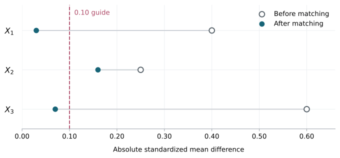
1. Which covariate shows the largest improvement in its absolute SMD?

2. Which covariate still exceeds the \(0.10\) rule of thumb after matching?

3. Identify one matching choice you could reconsider to address the remaining imbalance. What would you check after changing it, before estimating a causal effect?

8. Overlap and the causal target

A study has 100 treated people and 200 untreated people. Some treated people have no untreated people with sufficiently similar covariates. A matching analysis retains 70 treated people and uses 50 untreated people as their matches. The software reports the requested target as “ATT.”

1. Whose treatment effect does the resulting estimate concern? Explain why it need not estimate the ATT for all 100 treated people.

2. Suppose instead that all 100 treated people remain and the same 50 untreated people supply their matches, with reuse allowed. Does leaving out the 150 unused untreated people by itself change the ATT target? Explain.

9. What matching establishes

For each claim, state whether it is correct and explain your answer.

1. “Every covariate has an SMD of zero, so the covariate distributions must agree.”

2. “We used one untreated person as a match five times, so we have five independent untreated outcomes.”

Propensity scores

For these exercises, assume the measured-confounding SCM with binary exposure \(A\), outcome \(Y\), and covariates \(X\). Assume the observations are i.i.d. and the relevant conditional means are defined. Write \(E=e(X)\) for the true propensity score and \(\hat E=\hat e(X)\) for its estimate. In the outcome models, \(s\) denotes a numerical score value. You may use a calculator. Keep additional digits during calculations and report final answers to two decimal places.

10. Understanding the propensity score

Let \(X=(X_1,X_2)\), where both covariates are binary. The true propensity score is

\[ e(X)=0.10+0.20X_1+0.20X_2. \]

1. Calculate the propensity score for each covariate profile.

\(X_1\)	\(X_2\)	\(E=e(X)\)
0	0
0	1
1	0
1	1

2. Identify two different covariate profiles with the same propensity score.

3. Must two people with those profiles receive the same observed treatment? Explain.

11. Outcome regression with a continuous outcome

Return to the four people in Exercise 2, now with estimated propensity scores added. A fitted outcome regression using the score and treatment gives

\[ \hat\mu(s,a)=10+2s-3a-as. \]

1. Complete the prediction columns. Use each person’s estimated score as the score input, keeping it fixed when changing the treatment value.

\(X\)	\(A\)	\(\hat E\)	\(\hat\mu(\hat E,A)\)	\(\hat\mu(\hat E,1)\)	\(\hat\mu(\hat E,0)\)
1	0	0.20
2	1	0.40
3	0	0.60
4	1	0.80

2. Estimate \(E\left[Y(1)\right]\), \(E\left[Y(0)\right]\), and the ATE. Interpret the ATE in outcome units.

12. Outcome regression with a binary outcome

As in Exercise 3, \(Y\) is binary. A fitted outcome regression using the score and treatment gives

\[ \operatorname{logit}\{\hat\mu(s,a)\}=-1+s-a. \]

Consider four people with the estimated propensity scores shown below. To convert fitted log odds \(\eta\) to a probability, use \(\exp(\eta)/(1+\exp(\eta))\).

1. Complete the table. For each person, use their estimated score to predict the probability of \(Y=1\) under each treatment value.

Person	\(\hat E\)	\(\hat\mu(\hat E,1)\)	\(\hat\mu(\hat E,0)\)
1	0.25
2	0.25
3	0.75
4	0.75

2. Use the completed table to estimate \(E\left[Y(1)\right]\) and \(E\left[Y(0)\right]\) by averaging each prediction column.

3. Estimate and interpret the ATE, causal relative risk, and causal odds ratio for intervention value \(1\) compared with \(0\).

13. Propensity-score matching

Return to the data from Exercise 6, with estimated propensity scores added:

Person	\(X\)	\(A\)	\(Y\)	\(\hat E\)
1	1	1	8	0.20
2	2	0	5	0.30
3	4	1	15	0.80
4	8	0	11	0.70

1. Find one nearest untreated match for each treated person using absolute difference in estimated propensity scores. A person may be used as a match more than once. Complete the table using each treated person’s own outcome and their match’s outcome.

Treated person	Matched person	Estimate of \(\mu(\hat E,1)\)	Estimate of \(\mu(\hat E,0)\)	Difference
1
3

2. Estimate and interpret the ATT.

Inverse probability weighting

For these exercises, use the measured-confounding SCM with binary treatment \(A\). Use weighted means to estimate the intervention means. You may use a calculator; report final answers to two decimal places.

14. Who gets more weight?

For each study, say which person receives more weight for the specified intervention mean. Explain your reasoning without calculating weights.

1. In a study of a job-training program, people who are unemployed are more likely to enroll than people who are employed. Among two people who enrolled, one unemployed and one employed, whose outcome receives more weight when estimating mean earnings if everyone enrolled, \(E[Y(1)]\)?

2. In the same study, consider two people who did not enroll, one unemployed and one employed. Whose outcome receives more weight when estimating mean earnings if nobody enrolled, \(E[Y(0)]\)?

3. In a study of blood-pressure medication, people with more severe hypertension are more likely to receive medication. Among two people who received medication, whose outcome receives more weight when estimating mean blood pressure if everyone received medication, \(E[Y(1)]\): the person with more severe or less severe hypertension? Who receives more weight in estimating \(E[Y(0)]\) among two people who did not receive medication?

15. Computing an IPW estimate

Consider these four people, with true propensity scores supplied:

Person	\(X\)	\(A\)	\(Y\)	\(e(X)\)	Weight for \(E[Y(1)]\)	Weight for \(E[Y(0)]\)
Hickory	0	1	6	0.20
Hazel	0	0	4	0.20
Willow	1	1	10	0.80
Chestnut	1	0	8	0.80

1. Complete both weight columns, including the zero weights.

2. Estimate \(E[Y(1)]\), \(E[Y(0)]\), and the ATE using weighted means. Interpret the ATE.

16. Using a fitted propensity model

In a study of a training program, \(A=1\) denotes enrollment, \(X\) is the number of years unemployed before the program, and \(Y\) is earnings in thousands of dollars afterward. A fitted propensity model gives

\[ \operatorname{logit}\{\hat e(X)\}=X. \]

Convert fitted log odds \(\eta\) to a probability using \(\exp(\eta)/(1+\exp(\eta))\).

1. Use the fitted model to complete the estimated-score and weight columns, including zero weights.

Person	\(X\)	\(A\)	\(Y\)	\(\hat e(X)\)	Weight for \(E[Y(1)]\)	Weight for \(E[Y(0)]\)
Hickory	0	1	6
Hazel	0	0	4
Willow	1	1	10
Chestnut	1	0	8

2. Use weighted means to estimate \(E[Y(1)]\), \(E[Y(0)]\), and the ATE. Interpret the ATE.

17. Checking the scores and balance

The two panels below show estimated propensity score distributions in two studies. Each bar counts people in a score interval of width \(0.10\).

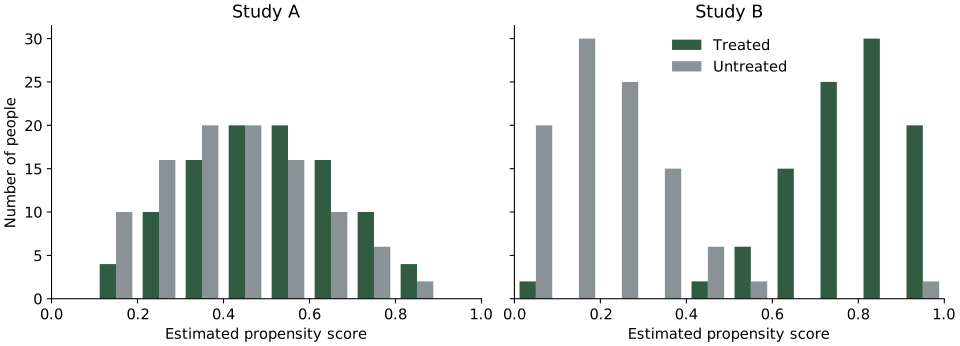
1. Which study has a more reassuring score distribution for IPW? In the other study, what should you watch out for?

2. In Study B, two treated people have estimated scores of \(0.01\) and two untreated people have estimated scores of \(0.99\). What weights do these people receive for estimating \(E[Y(1)]\) and \(E[Y(0)]\), respectively?

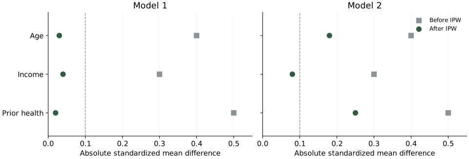
3. The balance plots below compare two fitted propensity models for the same study. Which model produces better covariate balance after IPW? Explain using the plotted values.

18. A different denominator

Return to Exercise 15. Compute the Horvitz–Thompson estimates of \(E[Y(1)]\), \(E[Y(0)]\), and the ATE by dividing each weighted outcome total by the number of people. Compare these with the weighted-mean estimates from Exercise 15.

Robust estimators

Use the working measured-confounding SCM from this section. All fitted predictions and model-assessment results needed for these exercises are supplied; no model fitting is required.

19. Computing an AIPW estimate

Two fitted models give the following propensity scores and outcome predictions:

Person	\(A\)	\(Y\)	\(\hat e(X)\)	\(\hat\mu(X,1)\)	\(\hat\mu(X,0)\)
Hickory	1	12	\(1/2\)	10	7
Hazel	0	6	\(1/4\)	9	7
Willow	1	8	\(3/4\)	9	6
Chestnut	0	10	\(1/2\)	11	8

1. Complete the IPW-weight, weighted-correction, and contribution columns for each treatment value, including zero weights and corrections.

Under treatment 1, the weighted correction is

\[ \frac{A}{\hat e(X)}\{Y-\hat\mu(X,1)\}. \]

Person	IPW weight \(A/\hat e(X)\)	Weighted correction	AIPW contribution
Hickory
Hazel
Willow
Chestnut

Under treatment 0, the weighted correction is

\[ \frac{1-A}{1-\hat e(X)}\{Y-\hat\mu(X,0)\}. \]

Person	IPW weight \((1-A)/(1-\hat e(X))\)	Weighted correction	AIPW contribution
Hickory
Hazel
Willow
Chestnut

2. Estimate \(E[Y(1)]\), \(E[Y(0)]\), and the ATE. Interpret the ATE.

20. What does robustness buy us?

1. A researcher fits additive linear and logistic models, then reports: “I used AIPW. It is doubly robust, so we can trust the estimate.” Explain what double robustness establishes and what you would still want to know about these fitted models.

2. Consider one covariate profile \(X=x\). The true and fitted functions are:

Function	True value	Fitted value
Outcome mean under treatment	\(\mu(x,1)=10\)	\(\hat\mu(x,1)=12\)
Propensity score	\(e(x)=0.40\)	\(\hat e(x)=0.50\)

Calculate the modeling bias at this covariate profile for outcome regression, IPW, and AIPW when estimating the mean under treatment. Use the Horvitz–Thompson form of IPW. Compare your results.

21. Choosing and using a flexible outcome model

The two panels show the same observations and two fitted outcome models. The circles and blue curves correspond to \(A=0\); the triangles and orange curves correspond to \(A=1\).

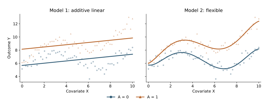
The models have the following mean squared prediction errors. Both were assessed using the same five cross-validation groups.

Model	Training error	Cross-validation error
1: additive linear	1.36	1.45
2: flexible	0.25	0.29

1. Describe one feature of the fitted relationship that Model 2 captures and Model 1 misses.

2. Which model would you select using the cross-validation results? Explain.

3. Describe how you would use the selected outcome model to estimate the ATE.