Exercises

A list of assignments

1. Telling a story

A study records three variables for each patient.

• Whether the patient has severe symptoms upon arriving at an emergency department
• Whether the patient receives diagnostic imaging
• Whether the patient is admitted to the hospital

Tell a story for how the world might generate these three variables. Write your story as a list. At each step, say which variable is generated and which other variables, if any, are used to generate it.

2. Generating one observation

Suppose the variables in the emergency-department study are generated according to the assignments

\[ X\leftarrow\operatorname{Bernoulli}(0.30), \]

\[ A\leftarrow\operatorname{Bernoulli}(0.15+0.65X), \]

\[ Y\leftarrow\operatorname{Bernoulli}(0.05+0.35X+0.15A). \]

Here, \(X\) indicates severe symptoms, \(A\) indicates diagnostic imaging, and \(Y\) indicates hospital admission. Write code that carries out these assignments and generates one observation \((X,A,Y)\). You may use R or another programming language. Explain why the lines of code must be run in the order you chose.

3. Finding topological orders

For each collection of assignments, find a topological order if one exists and determine whether it is unique. The order in which the assignments are displayed is not intended to be an order for generating the variables.

\[ Y\leftarrow\operatorname{Normal}(90+3X+2A,16), \]

\[ W\leftarrow\operatorname{Poisson}(3), \]

\[ A\leftarrow\operatorname{Binomial}\{4,\operatorname{logit}^{-1}(-1+0.2X+0.3W)\}, \]

\[ X\leftarrow\operatorname{Exponential}(1). \]

\[ A\leftarrow\operatorname{Poisson}\{\exp(0.1X+0.2W)\}, \]

\[ X\leftarrow\operatorname{Normal}(Y,1), \]

\[ W\leftarrow\operatorname{Bernoulli}(0.4), \]

\[ Y\leftarrow\operatorname{Normal}(5+A,4). \]

\[ W\leftarrow\operatorname{Normal}(2+X,1), \]

\[ Y\leftarrow\operatorname{Normal}(10+W+A,9), \]

\[ A\leftarrow\operatorname{Poisson}\{\exp(0.1W)\}, \]

\[ X\leftarrow\operatorname{Bernoulli}(0.5). \]

4. Decomposing a joint probability

Suppose \(X\) indicates whether a patient has severe asthma at baseline, \(Z\) indicates whether the patient’s insurance covers a controller medication, \(A\) indicates whether the patient uses the controller medication, and \(Y\) is the number of asthma exacerbations during the following year. Consider the assignments

\[ X\leftarrow\operatorname{Bernoulli}(0.5), \]

\[ Z\leftarrow\operatorname{Bernoulli}(0.4), \]

\[ A\leftarrow\operatorname{Bernoulli}(0.2+0.2X+0.2Z), \]

\[ Y\leftarrow\operatorname{Poisson}(2+X-A). \]

1. Use the assignments to find

\[ E[A\mid X,Z] \]

and

\[ E[Y\mid X,A]. \]

2. Use the assignments to decompose

\[ P(X=x,Z=z,A=a,Y=y). \]

For each factor, explain how the corresponding assignment tells you which variables belong after the conditioning bar.

3. Use your decomposition to calculate

\[ P(X=1,Z=0,A=1,Y=2). \]

Structural causal models

5. Writing structural causal models

For each story, write an SCM, state the parents of each variable, and state what must be true of the noise terms.

a. Wildfire smoke. Let \(X\) indicate unhealthy wildfire smoke, let \(A\) indicate whether a person stays indoors, and let \(Y\) indicate an asthma exacerbation. Staying indoors may depend on the smoke, and the outcome may depend on both the smoke and staying indoors.

b. Appointment-reminder trial. Suppose investigators randomly assign patients to receive an appointment reminder. Let \(X\) collect baseline characteristics, let \(A\) indicate randomized assignment to the reminder, let \(M\) indicate whether the patient attends the appointment, and let \(Y\) indicate whether blood pressure is measured at that appointment. Baseline characteristics may affect attendance and whether blood pressure is measured. The reminder may affect attendance. In this story, the reminder can affect whether blood pressure is measured only through attendance.

6. Using the local Markov property

Return to the wildfire-smoke and appointment-reminder SCMs. For each statement, determine whether we can use the local Markov property to conclude that it holds under the specified SCM. If we can, explain why and interpret the statement in context. If we cannot, explain why the local Markov property does not give us the statement.

1. In the wildfire-smoke SCM,

\[ A\mathrel{\perp\!\!\!\perp}X. \]

2. In the appointment-reminder SCM,

\[ A\mathrel{\perp\!\!\!\perp}X. \]

3. In the appointment-reminder SCM,

\[ M\mathrel{\perp\!\!\!\perp}A. \]

4. In the appointment-reminder SCM,

\[ Y\mathrel{\perp\!\!\!\perp}A\mid X,M. \]

7. Where might these SCMs be wrong?

Return to the SCMs you wrote for the wildfire-smoke story and the appointment-reminder trial. We emphasized two ways that an SCM can be wrong.

• The assignment function for a variable may be missing an important parent.
• The noise variables may not be independent because some shared input is hiding inside more than one of them.

For each story, give one concrete example of each problem. Be as specific as possible about the variable involved, which assignments would use it, and how you would revise the SCM.

a. Wildfire-smoke SCM

b. Appointment-reminder SCM

8. Following an SCM for one realization

Consider the SCM

\[ X\leftarrow\epsilon_X, \]

\[ A\leftarrow \begin{cases} 1, & \epsilon_A\leq 0.25+0.5X,\\ 0, & \epsilon_A>0.25+0.5X, \end{cases} \]

and

\[ Y\leftarrow X+2A+\epsilon_Y. \]

Suppose the noise variables have the realized values

\[ \epsilon_X=0.2, \qquad \epsilon_A=0.3, \qquad \epsilon_Y=0.4. \]

1. Follow the assignments in order. What values are placed into \(X\), \(A\), and \(Y\)?

2. Using the same values of \(X\) and \(\epsilon_Y\), define two new random variables

\[ Y_1=X+2(1)+\epsilon_Y \]

and

\[ Y_0=X+2(0)+\epsilon_Y. \]

What values do \(Y_1\) and \(Y_0\) take for this realization?

3. Compare \(Y\), \(Y_1\), and \(Y_0\). Which of the two new variables equals \(Y\)? Why? What is the difference \(Y_1-Y_0\)?

Causal graphs

9. Building a graph from an SCM

Consider the SCM

\[ \begin{aligned} W&\leftarrow f_W(\epsilon_W),\\ X&\leftarrow f_X(\epsilon_X),\\ A&\leftarrow f_A(W,X,\epsilon_A),\\ M&\leftarrow f_M(W,A,\epsilon_M),\\ Y&\leftarrow f_Y(X,M,\epsilon_Y), \end{aligned} \]

where the noise terms are independent.

1. Draw the causal graph.

2. List the parents of every variable.

10. Recovering an SCM from a graph

Consider the following causal graph.

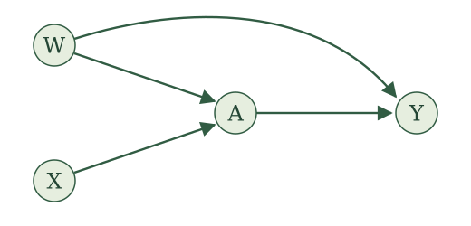
1. List the parents of every variable.

2. Write the SCM represented by the graph.

3. State what must be true of the noise terms.

11. Cycles and topological orders

For each graph, determine whether the corresponding SCM has a topological order. If it does, give one. If it does not, identify a directed cycle.

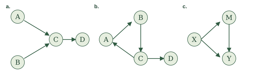
12. Using the graph for conditional independence

Return to the graph from Exercise 9 and use the topological order

\[ W,X,A,M,Y. \]

1. For each variable, identify the variables that appear earlier in the order but are not its parents.

2. Use the local Markov property to list every nontrivial conditional-independence statement supplied by this order.

3. Does the local Markov property tell us whether \(A\) and \(X\) are dependent? Does it tell us whether \(Y\) and \(W\) are conditionally dependent given \(X\)? Explain.

Global Markov property

13. Chest pain in the emergency department

Consider this made-up example. Among people experiencing chest pain in a region, rural residence and chest pain severity are independent. Let \(R\) indicate rural residence, \(Y\) denote chest pain severity before deciding whether to seek care, and \(S\) indicate whether a person visits the emergency department.

People living in rural areas face a longer journey to the emergency department and may stay home when symptoms are mild. More severe chest pain makes a visit more likely. These relationships are represented by the following graph:

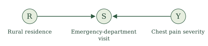
A researcher examines only emergency-department patients and finds that rural patients tend to have more severe chest pain. Explain how this association could arise even though rural residence and chest pain severity are independent in the regional population. Identify the variable being conditioned on and its role in the graph.

14. Listing and classifying paths

Consider the following causal graph.

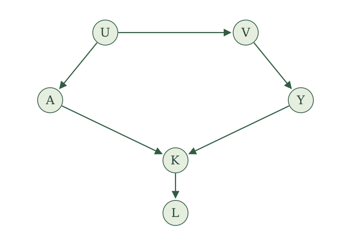
1. List every path between \(A\) and \(Y\).

2. For each path, state whether it is open or blocked when conditioning on nothing, on \(V\), and on \(V,L\). Identify the node responsible whenever a path is blocked.

15. Blocking individual paths

For each drawing, list all conditioning sets chosen from the displayed variables other than \(A,Y\) that block the specified path from \(A\) to \(Y\). Include the empty set if it works. Each drawing shows all relevant arrows.

1. \(A\leftarrow U\to V\to Y\).

2. \(A\to U\leftarrow V\leftarrow Y\).

3. \(A\to U\to V\leftarrow Y\), with the additional arrow \(V\to Z\). Study the path through \(U,V\); \(Z\) is not on it.

16. Finding d-separating sets

Return to the graph in Exercise 14. Choose conditioning variables only from \(U,V,K,L\).

1. Find two different conditioning sets that d-separate \(A\) and \(Y\). For each set, explain why every path is blocked.

2. Can a conditioning set containing \(K\) or \(L\) d-separate \(A\) and \(Y\)? Explain.

17. Applying the global Markov property

Suppose the graph in Exercise 14 comes from an SCM with a topological order.

1. Use your d-separation conclusions to state two conditional-independence relationships between \(A\) and \(Y\) guaranteed by the global Markov property.

2. Does the global Markov property guarantee \(A\perp Y\mid V,L\)? If not, does it establish that \(A\) and \(Y\) are conditionally dependent given \(V,L\)? Explain.

18. Conditioning on a variable measured before exposure

Consider the following causal graph. The variables \(W,U,V,M,T\) are measured before exposure \(A\). Suppose the graph comes from an SCM with a topological order.

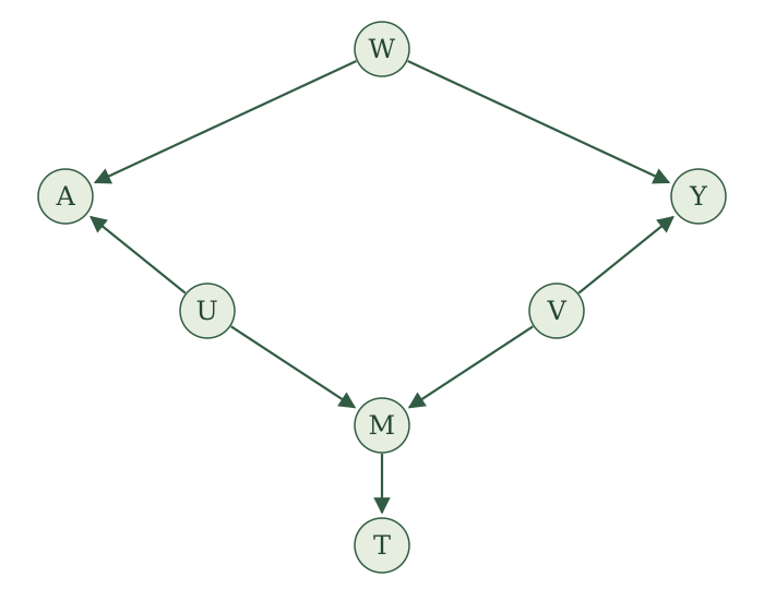
1. List every path between \(A\) and \(Y\). Does \(W\) d-separate them? State the corresponding conclusion from the global Markov property.

2. Does \(W,M\) d-separate \(A\) and \(Y\)? What about \(W,T\)? Explain what changes on each path.

3. A researcher argues that adding \(M\) to the conditioning collection is harmless because it was measured before \(A\). What does this graph tell us about that argument?

19. Can every path be blocked?

Consider the following causal graph from an SCM with a topological order.

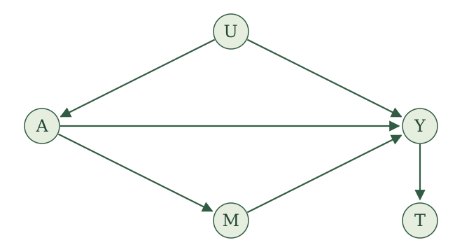
1. List every path between \(A\) and \(Y\). Which remain open conditional on \(U,M\)?

2. Can any collection chosen from \(U,M,T\) d-separate \(A\) and \(Y\)? Explain. Does your answer establish that \(A\) and \(Y\) are dependent?

20. Disconnected parts of a graph

Consider the following causal graph from an SCM with a topological order.

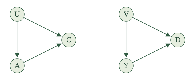
1. Are \(A\) and \(Y\) d-separated without conditioning? What does the global Markov property imply?

2. Are \(A\) and \(Y\) d-separated by \(C,D\)? Explain why conditioning on these colliders does or does not change your answer.

3. Does every collection chosen from \(U,V,C,D\) d-separate \(A\) and \(Y\)? Explain and state the general observation this illustrates.

Potential outcomes

21. Constructing potential outcomes

Suppose \(W\) is the outdoor wildfire-smoke level, \(A\) indicates whether a classroom air purifier is used, \(P\) is the indoor particulate level, and \(Y\) is the number of asthma symptoms reported by students. Consider the SCM

\[ \begin{aligned} W&\leftarrow f_W(\epsilon_W),\\ A&\leftarrow f_A(W,\epsilon_A),\\ P&\leftarrow f_P(W,A,\epsilon_P),\\ Y&\leftarrow f_Y(W,P,\epsilon_Y). \end{aligned} \]

For an intervention that sets purifier use to \(a\):

1. Rename every variable and write the resulting assignments before making the substitution.

2. Substitute \(a\) wherever \(A(a)\) appears on the right-hand side. Write the complete potential-outcome assignments.

3. The intervention value \(a\) does not appear explicitly in the final assignment for \(Y(a)\). Explain how it can nevertheless affect \(Y(a)\).

22. Applying causal irrelevance

Return to the air-purifier SCM in Exercise 21.

1. Consider \(W(a),A(a),P(a),Y(a)\) in assignment order. Which potential outcomes equal their original variables by causal irrelevance? Explain each conclusion by examining the variable’s parents, the parents of those parents, and so on.

2. Rewrite the complete potential-outcome assignments using every equality justified by causal irrelevance.

23. Applying consistency

Return again to the air-purifier SCM.

1. Suppose the original purifier value satisfies \(A=a\). Use the assignments in order to establish first that \(P(a)=P\) and then that \(Y(a)=Y\).

2. State the consistency conclusions separately for classrooms with \(A=1\) and classrooms with \(A=0\).

24. Calculating potential outcomes

Consider the SCM

\[ \begin{aligned} X&\leftarrow\epsilon_X,\\ A&\leftarrow\mathbb{1}(\epsilon_A<0.5),\\ Y&\leftarrow X+2A+\epsilon_Y. \end{aligned} \]

The following noise values have already been drawn:

Person	\(\epsilon_X\)	\(\epsilon_A\)	\(\epsilon_Y\)
1	0.2	0.3	0.4
2	0.8	0.7	0.1
3	0.5	0.2	0.6
4	0.1	0.9	0.8
5	0.6	0.4	0.2

1. Fill the eight missing cells in the table. Use the same row’s noise values to generate the original variables and all potential outcomes.

Person	\(X\)	\(A\)	\(Y\)	\(X(0)\)	\(A(0)\)	\(Y(0)\)	\(X(1)\)	\(A(1)\)	\(Y(1)\)
1	0.2	\(\square\)	2.6	0.2	1	\(\square\)	0.2	1	2.6
2	0.8	0	\(\square\)	0.8	0	0.9	0.8	0	2.9
3	0.5	1	3.1	\(\square\)	1	1.1	0.5	1	\(\square\)
4	0.1	0	0.9	0.1	\(\square\)	0.9	0.1	0	2.9
5	\(\square\)	1	2.8	0.6	1	\(\square\)	0.6	1	2.8

2. Which equalities in the completed table follow from causal irrelevance?

3. Verify consistency for each person. Which of \(Y(0)\) or \(Y(1)\) must equal \(Y\) in each row?

4. Calculate \(Y(1)-Y(0)\) for every person. What do you notice?

25. Three interventions over time

Suppose a patient’s insulin dose can be adjusted before breakfast, lunch, and dinner. Let \(A_j\) indicate whether an additional dose is given before meal \(j\), and let \(Y_j\) be the blood-glucose measurement after that meal. Consider the SCM

\[ \begin{aligned} A_1&\leftarrow f_{A_1}(\epsilon_{A_1}),\\ Y_1&\leftarrow f_{Y_1}(A_1,\epsilon_{Y_1}),\\ A_2&\leftarrow f_{A_2}(A_1,Y_1,\epsilon_{A_2}),\\ Y_2&\leftarrow f_{Y_2}(A_1,Y_1,A_2,\epsilon_{Y_2}),\\ A_3&\leftarrow f_{A_3}(A_1,Y_1,A_2,Y_2,\epsilon_{A_3}),\\ Y_3&\leftarrow f_{Y_3}(A_1,Y_1,A_2,Y_2,A_3,\epsilon_{Y_3}). \end{aligned} \]

1. Each treatment is binary. How many intervention combinations are possible?

2. Construct the complete potential-outcome assignments under \((a_1,a_2,a_3)=(1,0,1)\). Show the renaming step and the substitution step.

3. Apply causal irrelevance. Which potential outcomes can be replaced by their original variables?

4. Suppose only that \(A_1=1\). Which additional potential outcomes equal their original variables by consistency? Where does the equality stop?

5. Now suppose \(A_1=1\) and \(A_2=0\). Which additional equalities follow, and where does the equality stop next?

6. Finally, suppose \(A_1=1,A_2=0,A_3=1\). What does consistency imply about \(Y_3(1,0,1)\)?

26. Defining and interpreting causal effects

For each scenario:

1. write the causal effect using potential outcomes; and
2. interpret the supplied numerical value in context.

1. A smoking-cessation program is compared with no program. Let \(Y\) be the number of cigarettes smoked per day. The average treatment effect is \(-3.2\).

2. A vaccine is compared with no vaccine. Let \(Y\) indicate whether a person develops influenza. The causal relative risk is \(0.40\).

3. A pain therapy is compared with no therapy. Let \(Y\) be a pain score, and let the baseline variable \(X=1\) indicate severe pain before treatment. The average treatment effect among people with \(X=1\) is \(-5\).

4. An exercise program is compared with no program. Let \(Y\) be systolic blood pressure and let \(A\) indicate whether the person participated in the program in the original data-generating process. The average treatment effect among the treated is \(-6\).

Single-world intervention graphs

27. From assignments to a SWIG

Consider the potential-outcome SCM

\[ \begin{aligned} X(a)&\leftarrow f_X(\epsilon_X),\\ A(a)&\leftarrow f_A(X(a),\epsilon_A),\\ M(a)&\leftarrow f_M(X(a),a,\epsilon_M),\\ Y(a)&\leftarrow f_Y(a,M(a),\epsilon_Y). \end{aligned} \]

The noise terms are independent.

Draw its SWIG, including the fixed intervention value \(a\).

28. A single intervention from a causal graph

Consider the following causal graph:

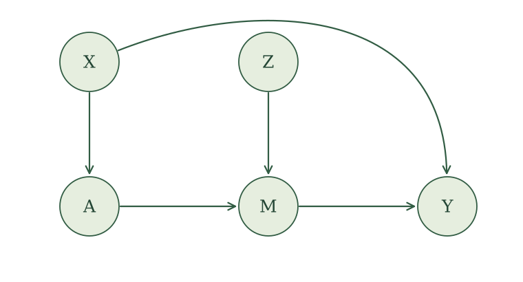
1. Construct the SWIG for an intervention on \(A\), with intervention value \(a\).

2. Apply causal irrelevance. Redraw the SWIG with simplified labels and explain each change.

3. For each statement below, decide whether it is guaranteed by the model. Explain using the local or global Markov property. When independence is not guaranteed, identify an open path.

\[ \begin{aligned} A&\mathrel{\perp\!\!\!\perp}Y(a),\\ A&\mathrel{\perp\!\!\!\perp}Y(a)\mid X,\\ A&\mathrel{\perp\!\!\!\perp}Y(a)\mid M(a). \end{aligned} \]

4. Decide whether each equality follows from the model. Explain which rule or rules justify it.

\[ E\left[Y(a)\mid A=a,X\right]=E\left[Y(a)\mid X\right], \]

\[ E\left[Y(a)\mid A=a,X\right]=E\left[Y\mid A=a,X\right]. \]

29. Multiple interventions

Consider the following causal graph:

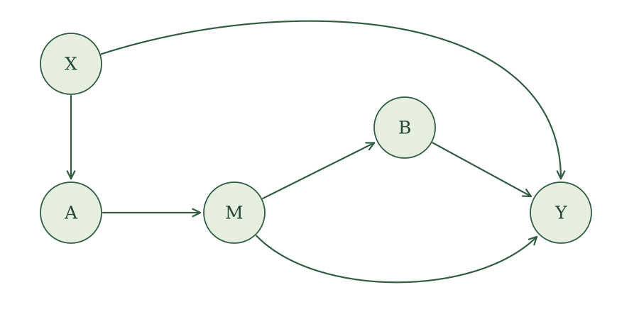
1. Construct the SWIG for interventions on both \(A\) and \(B\), with intervention values \(a\) and \(b\).

2. Apply causal irrelevance. Redraw the SWIG with simplified labels and explain each change.

3. For each statement below, decide whether it is guaranteed by the model. Explain using the local or global Markov property. When independence is not guaranteed, identify an open path.

\[ \begin{aligned} A&\mathrel{\perp\!\!\!\perp}Y(a,b)\mid X,\\ B(a)&\mathrel{\perp\!\!\!\perp}Y(a,b)\mid X,\\ B(a)&\mathrel{\perp\!\!\!\perp}Y(a,b)\mid X,M(a). \end{aligned} \]

4. Decide whether each equality follows from the model. Explain which rule or rules justify it.

\[ E\left[Y(a,b)\mid B(a)=b,X,M(a)\right] =E\left[Y(a,b)\mid X,M(a)\right], \]

\[ E\left[Y(a,b)\mid A=a,B=b,X\right] =E\left[Y\mid A=a,B=b,X\right]. \]