Sensitivity analyses for study 1

Pilot analysis using public NHANES data

Author

Amy Cochran

Sensitivity analyses

Pilot analysis

This rendered document currently uses public NHANES data with diabetes as the outcome to test the analysis workflow. It does not use SEED data and does not report results about autism. The sensitivity results shown here are pilot results and are not results from the planned autism analysis.

This document checks whether the conclusions from the primary analysis are sensitive to the number and length of the MCMC chains, the probit BART implementation, and unmeasured confounding. Each analysis changes one part of the primary analysis and examines whether the results remain stable.

Data preparation

The sensitivity analyses use the same analytic dataset and preprocessing steps as the primary analysis. We reproduce those steps here rather than loading a previously saved analytic dataset. This keeps the full data-processing workflow visible within the rendered document, allows us to repeat the associated data checks, and avoids creating additional files containing protected health information.

We first read the analysis configuration and source the shared functions used throughout the project. We then import the original data, assign the specified variable types, calculate the summaries needed to define contrasts for continuous predictors, create missingness indicators, impute missing values, and construct the final dataset supplied to the models. The same random seed and preprocessing sequence are used in the primary and sensitivity analyses so that both begin with the same realized analytic dataset.

# Source files
source("R/imports.R")

# Random seed
set.seed(20260322)

# Configuration
config <- yaml::read_yaml("config_1.yaml")

# Raw data and prepare data types
raw_df <- readr::read_csv(config$data_file)
prep <- coerce_variable_types(raw_df, config)
coerced_df <- prep$coerced_df
predictor_stats_df <- prep$predictor_stats_df

# Add in missingness indicators
prep <- add_missingness_indicators(
  coerced_df,
  config
)
indicated_df <- prep$indicated_df
final_config <- prep$config

# Impute remaining missing values
imputed_df <- impute_missing_data(
  indicated_df,
  final_config
)

# Final dataset
analytic_df <- finalize_analytic_dataset(
  imputed_df,
  final_config
)

Dropped 210 rows with missing outcome (diabetes).

# Remove objects we do not need
rm(
  raw_df,
  coerced_df,
  indicated_df,
  imputed_df,
  prep,
  config
)

Optional sandbox resampling

Sometimes we work with a sandbox dataset. This is not the dataset of scientific interest, but a stand-in used to run the full pipeline and see how it behaves. In that setting, we add one extra step. We resample cases and controls to a target size. The goal is to check whether the sample size is large enough for the analysis to be stable. This step is not part of the primary analysis.

# Optional sandbox-only resampling step

# Trigger when using the sandbox example (diabetes outcome)
is_sandbox_data <- identical(final_config$outcome$name, "diabetes")
cross_validation_group <- seq_len(nrow(analytic_df))

if (is_sandbox_data) {
  # Target sample sizes for cases and controls
  n_cases <- 2027
  n_controls <- 2696

  # Keep repeated copies of one original record in the same cross-validation
  # fold so that an identical record cannot occur in training and test data.
  analytic_df$.cross_validation_group <- seq_len(nrow(analytic_df))

  # Resample with replacement within outcome groups
  analytic_df <- dplyr::bind_rows(
    analytic_df |>
      dplyr::filter(.data[[final_config$outcome$name]] == 1) |>
      dplyr::slice_sample(n = n_cases, replace = TRUE),
    analytic_df |>
      dplyr::filter(.data[[final_config$outcome$name]] == 0) |>
      dplyr::slice_sample(n = n_controls, replace = TRUE)
  )

  cross_validation_group <- analytic_df$.cross_validation_group
  analytic_df$.cross_validation_group <- NULL

  # Inform the user that sandbox resampling was applied
  message("Sandbox resampling applied.")
}

Reference outcome model

We first fit the reference outcome model used in the primary analysis:

\[\Pr(Y = 1 \mid X, Z, S = 1).\]

This takes a while to fit, so we fit it once in this document and save it for later analyses. Retaining the trees allows us to reuse its posterior draws for prediction and sensitivity analyses.

# Prepare the outcome-model data
outcome_var <- final_config$outcome$name
predictor_vars <- vapply(final_config$predictors, `[[`, character(1), "name")
adjustment_vars <- setdiff(names(analytic_df), c(outcome_var, predictor_vars))

x_train <- analytic_df[, c(adjustment_vars, predictor_vars), drop = FALSE]
y_train <- analytic_df[[outcome_var]]

# Load the eight-chain reference model when available. Otherwise, fit and save
# it once for later renders.
dir.create("outputs/models", recursive = TRUE, showWarnings = FALSE)
set.seed(20260322)
reference_model_path <- "outputs/models/reference_outcome_bart.rds"

if (file.exists(reference_model_path)) {
  bart_fit <- readRDS(reference_model_path)
  reference_model_time <- NA_real_
} else {
  reference_model_time <- system.time({
    bart_fit <- dbarts::bart(
      x.train = x_train,
      y.train = y_train,
      keeptrees = TRUE,
      verbose = FALSE,
      nchain = 8L,
      nthread = 8L,
      nskip = 30000L,
      ndpost = 12000L,
      keepevery = 12L,
      seed = 20260322L
    )
  })[["elapsed"]]
  bart_fit$fit$storeState()
  saveRDS(bart_fit, reference_model_path)
}

The saved model should only be reused when the analytic data, variable definitions, and BART settings are unchanged. Because it contains information derived from the analytic sample, it should be stored with the same protections as the study data and should not be committed to version control.

Number and length of chains

We next examine how the allocation of a fixed sampling budget across chains affects the convergence diagnostics. The reference fit uses eight chains. We compare it with four longer chains and twelve shorter chains while holding approximately constant the total number of retained draws and total iterations. Thus, differences between the fits reflect how the same computational effort is distributed across chains rather than a larger sampling budget.

four_chain_path <- "outputs/models/four_chain_outcome_bart.rds"
twelve_chain_path <- "outputs/models/twelve_chain_outcome_bart.rds"

# Load each saved comparison when available. Otherwise, fit and save it once.
if (file.exists(four_chain_path)) {
  four_chain_fit <- readRDS(four_chain_path)
  four_chain_time <- NA_real_
} else {
  set.seed(20260322)
  four_chain_time <- system.time({
    four_chain_fit <- dbarts::bart(
      x.train = x_train,
      y.train = y_train,
      keeptrees = TRUE,
      verbose = FALSE,
      nchain = 4L,
      nthread = 4L,
      nskip = 60000L,
      ndpost = 24000L,
      keepevery = 12L,
      seed = 20260322L
    )
  })[["elapsed"]]
  four_chain_fit$fit$storeState()
  saveRDS(four_chain_fit, four_chain_path)
}

if (file.exists(twelve_chain_path)) {
  twelve_chain_fit <- readRDS(twelve_chain_path)
  twelve_chain_time <- NA_real_
} else {
  set.seed(20260322)
  twelve_chain_time <- system.time({
    twelve_chain_fit <- dbarts::bart(
      x.train = x_train,
      y.train = y_train,
      keeptrees = TRUE,
      verbose = FALSE,
      nchain = 12L,
      nthread = 10L,
      nskip = 20000L,
      ndpost = 8004L,
      keepevery = 12L,
      seed = 20260322L
    )
  })[["elapsed"]]
  twelve_chain_fit$fit$storeState()
  saveRDS(twelve_chain_fit, twelve_chain_path)
}

The three allocations retain approximately 8,000 draws and use approximately 336,000 total iterations. The twelve-chain allocation differs by only four retained draws and 48 iterations because each chain must retain a whole number of draws. Elapsed time is reported because distributing the iterations across more chains can change the computational cost even when the iteration budget is fixed.

chain_allocation_settings <- data.frame(
  allocation = c("4 longer chains", "8 reference chains", "12 shorter chains"),
  chains = c(4, 8, 12),
  threads = c(4, 8, 10),
  burnin_per_chain = c(60000, 30000, 20000),
  postburn_iterations_per_chain = c(24000, 12000, 8004),
  keep_every = c(12, 12, 12),
  retained_per_chain = c(2000, 1000, 667),
  total_retained = c(8000, 8000, 8004),
  total_iterations = c(336000, 336000, 336048),
  elapsed_seconds = c(four_chain_time, reference_model_time, twelve_chain_time)
)

chain_allocation_settings |>
  knitr::kable(
    digits = 1,
    col.names = c(
      "Allocation",
      "Chains",
      "Threads",
      "Burn-in per chain",
      "Post-burn iterations per chain",
      "Keep every",
      "Retained per chain",
      "Total retained",
      "Total iterations",
      "Elapsed seconds"
    ),
    caption = "Sampling effort and elapsed time by chain allocation"
  )

Sampling effort and elapsed time by chain allocation
Allocation	Chains	Threads	Burn-in per chain	Post-burn iterations per chain	Keep every	Retained per chain	Total retained	Total iterations	Elapsed seconds
4 longer chains	4	4	60000	24000	12	2000	8000	336000	NA
8 reference chains	8	8	30000	12000	12	1000	8000	336000	NA
12 shorter chains	12	10	20000	8004	12	667	8004	336048	NA

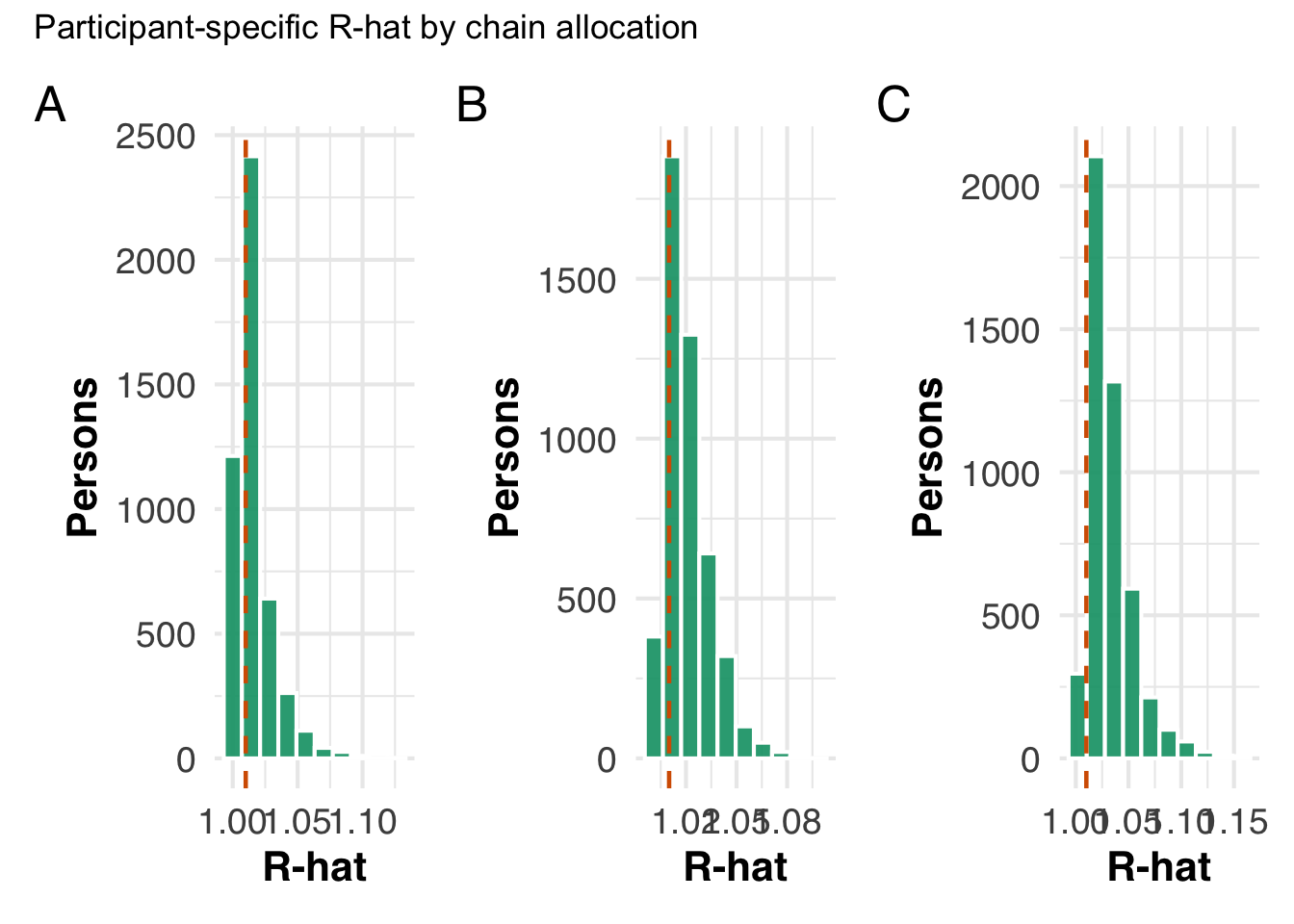
We apply the same diagnostics to all three fits. The global diagnostic follows the mean fitted probability across iterations. The participant-specific diagnostic calculates R-hat separately for every fitted probability. We use the maximum of rank-normalized split R-hat and rank-normalized folded-split R-hat, which is sensitive to differences in both the locations and scales of the chain distributions.

four_chain_diagnostics <- model_diagnostics(
  bart_fit = four_chain_fit,
  analytic_df = analytic_df,
  outcome_var = outcome_var,
  save_path = "outputs/diagnostics/chain_allocation/four_chains",
  nchain = 4L,
  ndpost = 2000L
)

eight_chain_diagnostics <- model_diagnostics(
  bart_fit = bart_fit,
  analytic_df = analytic_df,
  outcome_var = outcome_var,
  save_path = "outputs/diagnostics/reference",
  nchain = 8L,
  ndpost = 1000L
)

twelve_chain_diagnostics <- model_diagnostics(
  bart_fit = twelve_chain_fit,
  analytic_df = analytic_df,
  outcome_var = outcome_var,
  save_path = "outputs/diagnostics/chain_allocation/twelve_chains",
  nchain = 12L,
  ndpost = 667L
)

The global summary compares R-hat, bulk effective sample size, and tail effective sample size for the mean fitted probability. Bulk ESS describes the information available for central posterior summaries, while tail ESS describes the information available for posterior quantiles.

global_chain_diagnostics <- dplyr::bind_rows(
  transform(
    four_chain_diagnostics$ess_summary,
    allocation = "4 longer chains"
  ),
  transform(
    eight_chain_diagnostics$ess_summary,
    allocation = "8 reference chains"
  ),
  transform(
    twelve_chain_diagnostics$ess_summary,
    allocation = "12 shorter chains"
  )
) |>
  dplyr::select(
    allocation,
    rhat,
    ess_bulk,
    ess_tail,
    ess_bulk_per_chain,
    ess_tail_per_chain
  )

global_chain_diagnostics |>
  knitr::kable(
    digits = 3,
    col.names = c(
      "Allocation",
      "R-hat",
      "Bulk ESS",
      "Tail ESS",
      "Bulk ESS per chain",
      "Tail ESS per chain"
    ),
    caption = "Diagnostics for the mean fitted probability"
  )

Diagnostics for the mean fitted probability
Allocation	R-hat	Bulk ESS	Tail ESS	Bulk ESS per chain	Tail ESS per chain
4 longer chains	1.001	8245.278	8099.519	2061.320	2024.880
8 reference chains	1.000	7882.388	7595.044	985.299	949.381
12 shorter chains	1.001	8093.049	8203.244	674.421	683.604

For the participant-specific fitted probabilities, we report the full R-hat summary and the proportions below 1.05, 1.10, and 1.20. We consider the individual diagnostics adequate when the median is below 1.05, at least 90% are below 1.10, and at least 99% are below 1.20. We report the maximum but do not allow one individual value to determine the overall result.

participant_rhat_summary <- dplyr::bind_rows(
  transform(
    four_chain_diagnostics$rhat_summary,
    allocation = "4 longer chains"
  ),
  transform(
    eight_chain_diagnostics$rhat_summary,
    allocation = "8 reference chains"
  ),
  transform(
    twelve_chain_diagnostics$rhat_summary,
    allocation = "12 shorter chains"
  )
) |>
  dplyr::select(allocation, quantity, value)

rhat_reference_values <- c(1.05, 1.10, 1.20)
rhat_proportions <- dplyr::bind_rows(
  data.frame(
    allocation = "4 longer chains",
    threshold = rhat_reference_values,
    proportion_below = vapply(
      rhat_reference_values,
      function(value) mean(four_chain_diagnostics$rhat_values < value),
      numeric(1)
    )
  ),
  data.frame(
    allocation = "8 reference chains",
    threshold = rhat_reference_values,
    proportion_below = vapply(
      rhat_reference_values,
      function(value) mean(eight_chain_diagnostics$rhat_values < value),
      numeric(1)
    )
  ),
  data.frame(
    allocation = "12 shorter chains",
    threshold = rhat_reference_values,
    proportion_below = vapply(
      rhat_reference_values,
      function(value) mean(twelve_chain_diagnostics$rhat_values < value),
      numeric(1)
    )
  )
)

participant_rhat_summary |>
  knitr::kable(
    digits = 3,
    col.names = c("Allocation", "Summary", "R-hat"),
    caption = "Distribution of participant-specific R-hat values"
  )

Distribution of participant-specific R-hat values
Allocation	Summary	R-hat
4 longer chains	min	1.000
4 longer chains	q1	1.007
4 longer chains	median	1.012
4 longer chains	mean	1.016
4 longer chains	q3	1.020
4 longer chains	max	1.126
8 reference chains	min	1.001
8 reference chains	q1	1.012
8 reference chains	median	1.018
8 reference chains	mean	1.021
8 reference chains	q3	1.027
8 reference chains	max	1.098
12 shorter chains	min	1.002
12 shorter chains	q1	1.018
12 shorter chains	median	1.027
12 shorter chains	mean	1.033
12 shorter chains	q3	1.041
12 shorter chains	max	1.157

rhat_proportions |>
  knitr::kable(
    digits = 3,
    col.names = c("Allocation", "R-hat threshold", "Proportion below"),
    caption = "Participant-specific R-hat values below reference thresholds"
  )

Participant-specific R-hat values below reference thresholds
Allocation	R-hat threshold	Proportion below
4 longer chains	1.05	0.963
4 longer chains	1.10	0.999
4 longer chains	1.20	1.000
8 reference chains	1.05	0.966
8 reference chains	1.10	1.000
8 reference chains	1.20	1.000
12 shorter chains	1.05	0.838
12 shorter chains	1.10	0.982
12 shorter chains	1.20	1.000

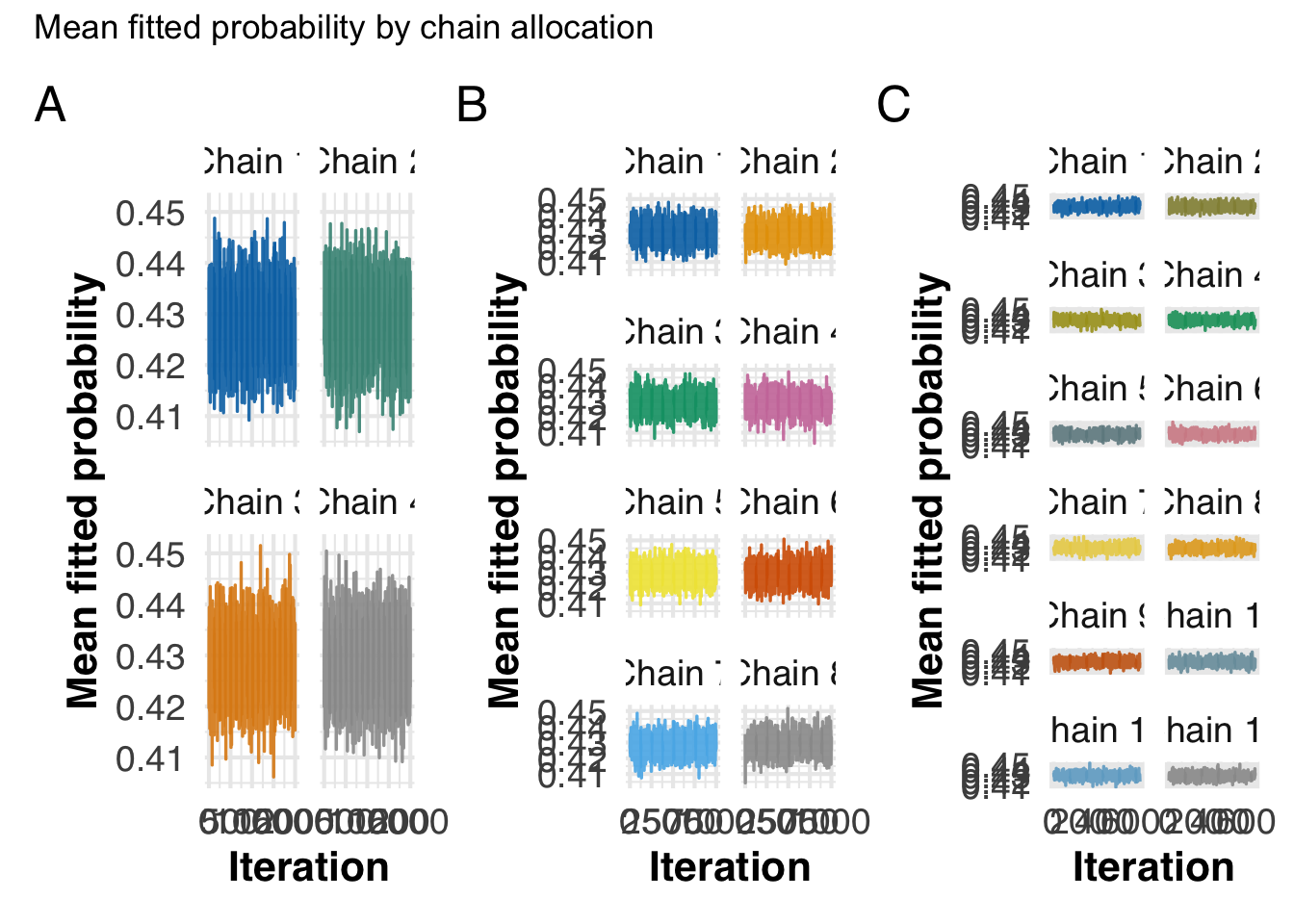
The histograms show the complete participant-specific R-hat distributions, and the trace plots show the mean fitted probability within each chain.

four_chain_diagnostics$plots$rhat +
  eight_chain_diagnostics$plots$rhat +
  twelve_chain_diagnostics$plots$rhat +
  patchwork::plot_annotation(
    tag_levels = "A",
    title = "Participant-specific R-hat by chain allocation"
  )

four_chain_diagnostics$plots$trace +
  eight_chain_diagnostics$plots$trace +
  twelve_chain_diagnostics$plots$trace +
  patchwork::plot_annotation(
    tag_levels = "A",
    title = "Mean fitted probability by chain allocation"
  )

The alternative fit is removed after its diagnostics are calculated because the saved tree object is large and is not needed in the remaining sensitivity analyses.

rm(four_chain_fit, twelve_chain_fit)
gc()

            used   (Mb) gc trigger   (Mb) limit (Mb)  max used   (Mb)
Ncells   3431213  183.3    5414985  289.2         NA   5414985  289.2
Vcells 171147673 1305.8  260736875 1989.3      24576 260736875 1989.3

Comparison of probit BART implementations

Before changing the assumptions of the model, we compare four probit BART implementations: BART, the bart() and bart2() interfaces from dbarts, and flexBART. All four use the same analytic data and probit link. We use the same number of chains, burn-in iterations, and retained draws so that Monte Carlo effort is comparable. Each package otherwise retains its ordinary defaults, including its number of trees, function prior, and variable-selection prior. This allows us to assess whether those implementation choices meaningfully change the PRRs. The reference model supplies the dbarts::bart result. We fit the other three models here and save them with their recorded fitting times.

BART and dbarts::bart represent categorical variables through indicator columns. dbarts::bart2 uses the package’s formula interface. flexBART receives the original data frame and handles categorical variables directly. Its optional nesting extensions are disabled, so all three packages fit the same basic binary probit BART model. Differences in their ordinary priors, cutpoint construction, and categorical splitting remain part of the comparison.

We deliberately retain the model defaults of each function. Thus, BART and flexBART use 50 trees, dbarts::bart uses 200 trees, and dbarts::bart2 uses 75 trees. We also leave their ordinary prior settings unchanged, including the family-specific default for k in bart2(). We override only the number and length of chains, thinning, parallelization, random seed, and whether trees and training fits are saved. The latter settings affect computation and stored output rather than the fitted model specification.

comparison_model_path <- "outputs/models/probit_bart_comparison.rds"

if (file.exists(comparison_model_path)) {
  comparison_fits <- readRDS(comparison_model_path)
} else {
  comparison_fits <- fit_probit_bart_comparison(
    analytic_df = analytic_df,
    outcome_var = final_config$outcome$name,
    nchain = 8L,
    nskip = 30000L,
    ndpost = 1000L,
    thin = 12L,
    seed = 20260322L
  )

  comparison_fits$dbarts_bart2$fit$storeState()
  saveRDS(comparison_fits, comparison_model_path)
}

All four implementations use eight chains, 30,000 burn-in iterations per chain, and 12,000 post-burn iterations per chain. Every twelfth post-burn draw is retained, giving 1,000 retained draws per chain. All chains run in parallel.

software_settings <- data.frame(
  software = c("BART", "dbarts::bart", "dbarts::bart2", "flexBART"),
  chains = c(8, 8, 8, 8),
  burnin_per_chain = c(30000, 30000, 30000, 30000),
  postburn_iterations_per_chain = c(12000, 12000, 12000, 12000),
  keep_every = c(12, 12, 12, 12),
  retained_per_chain = c(1000, 1000, 1000, 1000),
  parallel_chains = c(8, 8, 8, 8)
)

software_settings |>
  knitr::kable(
    col.names = c(
      "Software",
      "Chains",
      "Burn-in per chain",
      "Post-burn iterations per chain",
      "Keep every",
      "Retained per chain",
      "Parallel chains"
    ),
    caption = "Sampling settings for the software comparison"
  )

Sampling settings for the software comparison
Software	Chains	Burn-in per chain	Post-burn iterations per chain	Keep every	Retained per chain	Parallel chains
BART	8	30000	12000	12	1000	8
dbarts::bart	8	30000	12000	12	1000	8
dbarts::bart2	8	30000	12000	12	1000	8
flexBART	8	30000	12000	12	1000	8

We apply the same participant-specific convergence criteria to each software implementation. We also report diagnostics for the mean fitted probability and two measures of predictive accuracy: the Brier score and negative log probability. Lower values indicate better predictions for both measures.

software_diagnostic_results <- comparison_model_diagnostics(
  fits = comparison_fits,
  reference_model = bart_fit,
  analytic_df = analytic_df,
  outcome_var = outcome_var,
  save_path = "outputs/diagnostics/software_comparison",
  reference_save_path = "outputs/diagnostics/reference"
)

software_diagnostics <- software_diagnostic_results$summary

software_diagnostics$adequate_individual_diagnostics <- with(
  software_diagnostics,
  median_individual_rhat < 1.05 &
    proportion_below_1.10 >= 0.90 &
    proportion_below_1.20 >= 0.99
)

readr::write_csv(
  software_diagnostics,
  "outputs/diagnostics/software_comparison/summary.csv"
)

software_diagnostics |>
  knitr::kable(
    digits = 3,
    col.names = c(
      "Software",
      "Median individual R-hat",
      "Proportion below 1.10",
      "Proportion below 1.20",
      "Maximum individual R-hat",
      "Global R-hat",
      "Bulk ESS",
      "Tail ESS",
      "Brier score",
      "Negative log probability",
      "Meets individual criteria"
    ),
    caption = "Diagnostics for the probit BART implementations"
  )

Diagnostics for the probit BART implementations
Software	Median individual R-hat	Proportion below 1.10	Proportion below 1.20	Maximum individual R-hat	Global R-hat	Bulk ESS	Tail ESS	Brier score	Negative log probability	Meets individual criteria
BART	1.175	0.166	0.606	1.717	1.001	7861.309	7936.192	0.174	0.523	FALSE
dbarts::bart	1.018	1.000	1.000	1.098	1.000	7882.388	7595.044	0.180	0.536	TRUE
dbarts::bart2	1.283	0.055	0.288	2.101	1.000	7878.761	7615.151	0.156	0.476	FALSE
flexBART	1.108	0.440	0.865	1.618	1.000	8069.298	7641.941	0.179	0.534	FALSE

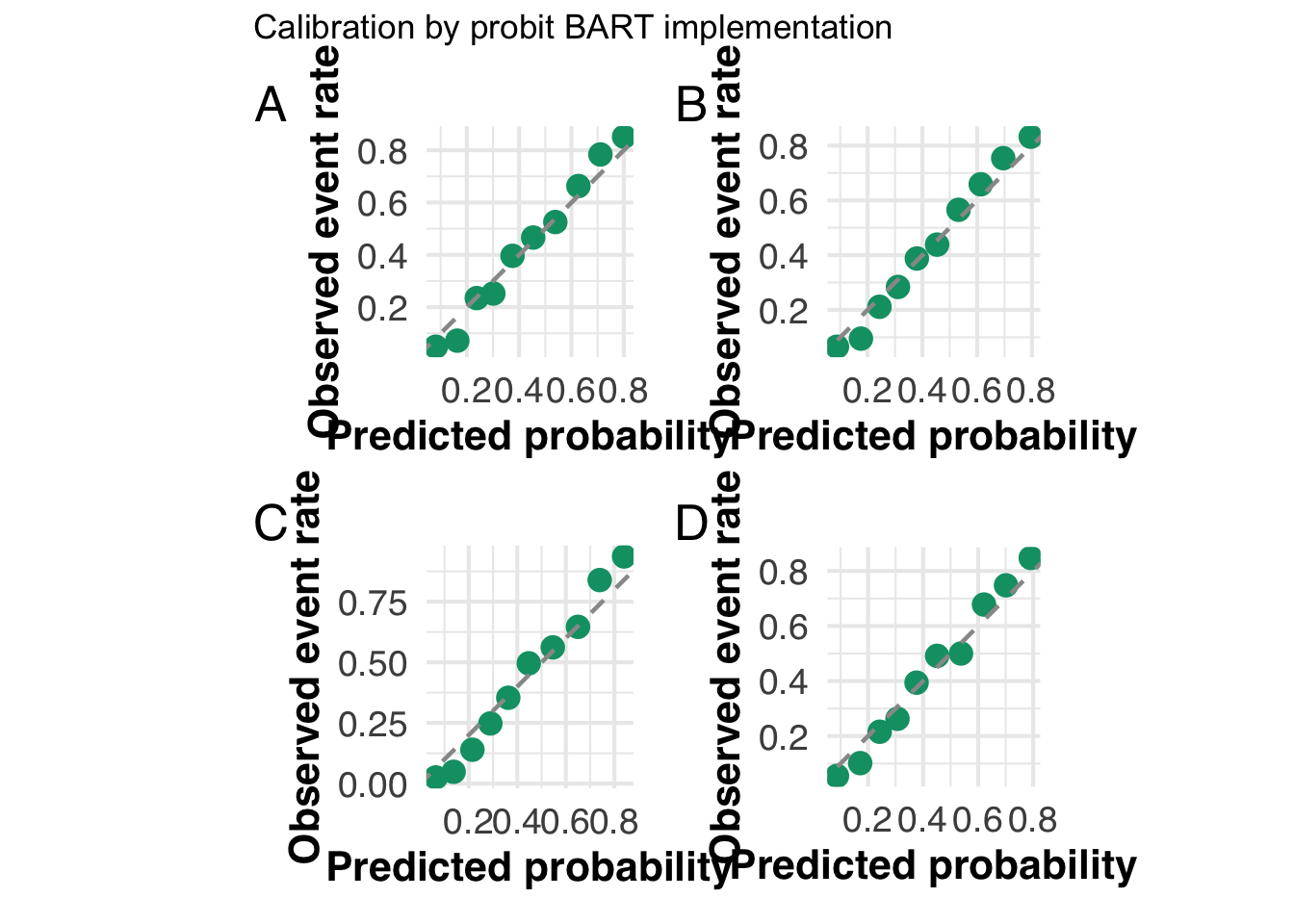
The calibration plots use the posterior mean predicted probability for each person and compare predicted and observed event rates within tenths of predicted risk.

software_diagnostic_results$diagnostics$BART$plots$calib +
  software_diagnostic_results$diagnostics$dbarts_bart$plots$calib +
  software_diagnostic_results$diagnostics$dbarts_bart2$plots$calib +
  software_diagnostic_results$diagnostics$flexBART$plots$calib +
  patchwork::plot_annotation(
    tag_levels = "A",
    title = "Calibration by probit BART implementation"
  )

Elapsed time includes the complete set of chains for each implementation. These times describe computational cost on the machine used to render this document; they are not measures of statistical performance. The reference-model time is shown as missing when that saved model is loaded rather than fitted during the current render.

software_timing <- rbind(
  data.frame(
    software = "dbarts::bart",
    elapsed_seconds = reference_model_time
  ),
  comparison_fits$timing
)

software_timing |>
  knitr::kable(
    digits = 1,
    col.names = c("Software", "Elapsed seconds"),
    caption = "Elapsed time for fitting the probit BART models"
  )

Elapsed time for fitting the probit BART models
Software	Elapsed seconds
dbarts::bart	NA
BART	592.2
dbarts::bart2	192.4
flexBART	124.0

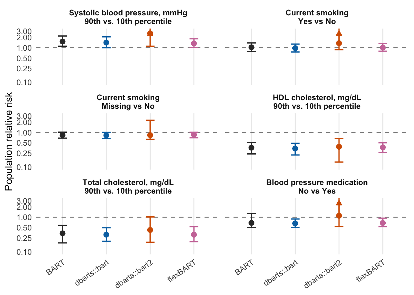
For each fitted model, we calculate the same population relative risks used in the primary analysis. Categorical predictors compare each level with the most common observed level; continuous predictors compare the 90th with the 10th percentile. The models are therefore compared on the primary target estimand, not merely on their fitted probabilities.

software_prrs <- compare_bart_prrs(
  fits = comparison_fits,
  reference_model = bart_fit,
  analytic_df = analytic_df,
  config = final_config,
  predictor_stats_df = predictor_stats_df
)

*****In main of C++ for bart prediction
tc (threadcount): 1
number of bart draws: 1000
number of trees in bart sum: 50
number of x columns: 11
from x,np,p: 11, 4723
***using serial code
*****In main of C++ for bart prediction
tc (threadcount): 1
number of bart draws: 1000
number of trees in bart sum: 50
number of x columns: 11
from x,np,p: 11, 4723
***using serial code
*****In main of C++ for bart prediction
tc (threadcount): 1
number of bart draws: 1000
number of trees in bart sum: 50
number of x columns: 11
from x,np,p: 11, 4723
***using serial code
*****In main of C++ for bart prediction
tc (threadcount): 1
number of bart draws: 1000
number of trees in bart sum: 50
number of x columns: 11
from x,np,p: 11, 4723
***using serial code
*****In main of C++ for bart prediction
tc (threadcount): 1
number of bart draws: 1000
number of trees in bart sum: 50
number of x columns: 11
from x,np,p: 11, 4723
***using serial code
*****In main of C++ for bart prediction
tc (threadcount): 1
number of bart draws: 1000
number of trees in bart sum: 50
number of x columns: 11
from x,np,p: 11, 4723
***using serial code
*****In main of C++ for bart prediction
tc (threadcount): 1
number of bart draws: 1000
number of trees in bart sum: 50
number of x columns: 11
from x,np,p: 11, 4723
***using serial code
*****In main of C++ for bart prediction
tc (threadcount): 1
number of bart draws: 1000
number of trees in bart sum: 50
number of x columns: 11
from x,np,p: 11, 4723
***using serial code
*****In main of C++ for bart prediction
tc (threadcount): 1
number of bart draws: 1000
number of trees in bart sum: 50
number of x columns: 11
from x,np,p: 11, 4723
***using serial code
*****In main of C++ for bart prediction
tc (threadcount): 1
number of bart draws: 1000
number of trees in bart sum: 50
number of x columns: 11
from x,np,p: 11, 4723
***using serial code
*****In main of C++ for bart prediction
tc (threadcount): 1
number of bart draws: 1000
number of trees in bart sum: 50
number of x columns: 11
from x,np,p: 11, 4723
***using serial code
*****In main of C++ for bart prediction
tc (threadcount): 1
number of bart draws: 1000
number of trees in bart sum: 50
number of x columns: 11
from x,np,p: 11, 4723
***using serial code
*****In main of C++ for bart prediction
tc (threadcount): 1
number of bart draws: 1000
number of trees in bart sum: 50
number of x columns: 11
from x,np,p: 11, 4723
***using serial code
*****In main of C++ for bart prediction
tc (threadcount): 1
number of bart draws: 1000
number of trees in bart sum: 50
number of x columns: 11
from x,np,p: 11, 4723
***using serial code
*****In main of C++ for bart prediction
tc (threadcount): 1
number of bart draws: 1000
number of trees in bart sum: 50
number of x columns: 11
from x,np,p: 11, 4723
***using serial code
*****In main of C++ for bart prediction
tc (threadcount): 1
number of bart draws: 1000
number of trees in bart sum: 50
number of x columns: 11
from x,np,p: 11, 4723
***using serial code
*****In main of C++ for bart prediction
tc (threadcount): 1
number of bart draws: 1000
number of trees in bart sum: 50
number of x columns: 11
from x,np,p: 11, 4723
***using serial code
*****In main of C++ for bart prediction
tc (threadcount): 1
number of bart draws: 1000
number of trees in bart sum: 50
number of x columns: 11
from x,np,p: 11, 4723
***using serial code
*****In main of C++ for bart prediction
tc (threadcount): 1
number of bart draws: 1000
number of trees in bart sum: 50
number of x columns: 11
from x,np,p: 11, 4723
***using serial code
*****In main of C++ for bart prediction
tc (threadcount): 1
number of bart draws: 1000
number of trees in bart sum: 50
number of x columns: 11
from x,np,p: 11, 4723
***using serial code
*****In main of C++ for bart prediction
tc (threadcount): 1
number of bart draws: 1000
number of trees in bart sum: 50
number of x columns: 11
from x,np,p: 11, 4723
***using serial code
*****In main of C++ for bart prediction
tc (threadcount): 1
number of bart draws: 1000
number of trees in bart sum: 50
number of x columns: 11
from x,np,p: 11, 4723
***using serial code
*****In main of C++ for bart prediction
tc (threadcount): 1
number of bart draws: 1000
number of trees in bart sum: 50
number of x columns: 11
from x,np,p: 11, 4723
***using serial code
*****In main of C++ for bart prediction
tc (threadcount): 1
number of bart draws: 1000
number of trees in bart sum: 50
number of x columns: 11
from x,np,p: 11, 4723
***using serial code
*****In main of C++ for bart prediction
tc (threadcount): 1
number of bart draws: 1000
number of trees in bart sum: 50
number of x columns: 11
from x,np,p: 11, 4723
***using serial code
*****In main of C++ for bart prediction
tc (threadcount): 1
number of bart draws: 1000
number of trees in bart sum: 50
number of x columns: 11
from x,np,p: 11, 4723
***using serial code
*****In main of C++ for bart prediction
tc (threadcount): 1
number of bart draws: 1000
number of trees in bart sum: 50
number of x columns: 11
from x,np,p: 11, 4723
***using serial code
*****In main of C++ for bart prediction
tc (threadcount): 1
number of bart draws: 1000
number of trees in bart sum: 50
number of x columns: 11
from x,np,p: 11, 4723
***using serial code
*****In main of C++ for bart prediction
tc (threadcount): 1
number of bart draws: 1000
number of trees in bart sum: 50
number of x columns: 11
from x,np,p: 11, 4723
***using serial code
*****In main of C++ for bart prediction
tc (threadcount): 1
number of bart draws: 1000
number of trees in bart sum: 50
number of x columns: 11
from x,np,p: 11, 4723
***using serial code
*****In main of C++ for bart prediction
tc (threadcount): 1
number of bart draws: 1000
number of trees in bart sum: 50
number of x columns: 11
from x,np,p: 11, 4723
***using serial code
*****In main of C++ for bart prediction
tc (threadcount): 1
number of bart draws: 1000
number of trees in bart sum: 50
number of x columns: 11
from x,np,p: 11, 4723
***using serial code
*****In main of C++ for bart prediction
tc (threadcount): 1
number of bart draws: 1000
number of trees in bart sum: 50
number of x columns: 11
from x,np,p: 11, 4723
***using serial code
*****In main of C++ for bart prediction
tc (threadcount): 1
number of bart draws: 1000
number of trees in bart sum: 50
number of x columns: 11
from x,np,p: 11, 4723
***using serial code
*****In main of C++ for bart prediction
tc (threadcount): 1
number of bart draws: 1000
number of trees in bart sum: 50
number of x columns: 11
from x,np,p: 11, 4723
***using serial code
*****In main of C++ for bart prediction
tc (threadcount): 1
number of bart draws: 1000
number of trees in bart sum: 50
number of x columns: 11
from x,np,p: 11, 4723
***using serial code
*****In main of C++ for bart prediction
tc (threadcount): 1
number of bart draws: 1000
number of trees in bart sum: 50
number of x columns: 11
from x,np,p: 11, 4723
***using serial code
*****In main of C++ for bart prediction
tc (threadcount): 1
number of bart draws: 1000
number of trees in bart sum: 50
number of x columns: 11
from x,np,p: 11, 4723
***using serial code
*****In main of C++ for bart prediction
tc (threadcount): 1
number of bart draws: 1000
number of trees in bart sum: 50
number of x columns: 11
from x,np,p: 11, 4723
***using serial code
*****In main of C++ for bart prediction
tc (threadcount): 1
number of bart draws: 1000
number of trees in bart sum: 50
number of x columns: 11
from x,np,p: 11, 4723
***using serial code
*****In main of C++ for bart prediction
tc (threadcount): 1
number of bart draws: 1000
number of trees in bart sum: 50
number of x columns: 11
from x,np,p: 11, 4723
***using serial code
*****In main of C++ for bart prediction
tc (threadcount): 1
number of bart draws: 1000
number of trees in bart sum: 50
number of x columns: 11
from x,np,p: 11, 4723
***using serial code
*****In main of C++ for bart prediction
tc (threadcount): 1
number of bart draws: 1000
number of trees in bart sum: 50
number of x columns: 11
from x,np,p: 11, 4723
***using serial code
*****In main of C++ for bart prediction
tc (threadcount): 1
number of bart draws: 1000
number of trees in bart sum: 50
number of x columns: 11
from x,np,p: 11, 4723
***using serial code
*****In main of C++ for bart prediction
tc (threadcount): 1
number of bart draws: 1000
number of trees in bart sum: 50
number of x columns: 11
from x,np,p: 11, 4723
***using serial code
*****In main of C++ for bart prediction
tc (threadcount): 1
number of bart draws: 1000
number of trees in bart sum: 50
number of x columns: 11
from x,np,p: 11, 4723
***using serial code
*****In main of C++ for bart prediction
tc (threadcount): 1
number of bart draws: 1000
number of trees in bart sum: 50
number of x columns: 11
from x,np,p: 11, 4723
***using serial code
*****In main of C++ for bart prediction
tc (threadcount): 1
number of bart draws: 1000
number of trees in bart sum: 50
number of x columns: 11
from x,np,p: 11, 4723
***using serial code
*****In main of C++ for bart prediction
tc (threadcount): 1
number of bart draws: 1000
number of trees in bart sum: 50
number of x columns: 11
from x,np,p: 11, 4723
***using serial code
*****In main of C++ for bart prediction
tc (threadcount): 1
number of bart draws: 1000
number of trees in bart sum: 50
number of x columns: 11
from x,np,p: 11, 4723
***using serial code
*****In main of C++ for bart prediction
tc (threadcount): 1
number of bart draws: 1000
number of trees in bart sum: 50
number of x columns: 11
from x,np,p: 11, 4723
***using serial code
*****In main of C++ for bart prediction
tc (threadcount): 1
number of bart draws: 1000
number of trees in bart sum: 50
number of x columns: 11
from x,np,p: 11, 4723
***using serial code
*****In main of C++ for bart prediction
tc (threadcount): 1
number of bart draws: 1000
number of trees in bart sum: 50
number of x columns: 11
from x,np,p: 11, 4723
***using serial code
*****In main of C++ for bart prediction
tc (threadcount): 1
number of bart draws: 1000
number of trees in bart sum: 50
number of x columns: 11
from x,np,p: 11, 4723
***using serial code
*****In main of C++ for bart prediction
tc (threadcount): 1
number of bart draws: 1000
number of trees in bart sum: 50
number of x columns: 11
from x,np,p: 11, 4723
***using serial code
*****In main of C++ for bart prediction
tc (threadcount): 1
number of bart draws: 1000
number of trees in bart sum: 50
number of x columns: 11
from x,np,p: 11, 4723
***using serial code
*****In main of C++ for bart prediction
tc (threadcount): 1
number of bart draws: 1000
number of trees in bart sum: 50
number of x columns: 11
from x,np,p: 11, 4723
***using serial code
*****In main of C++ for bart prediction
tc (threadcount): 1
number of bart draws: 1000
number of trees in bart sum: 50
number of x columns: 11
from x,np,p: 11, 4723
***using serial code
*****In main of C++ for bart prediction
tc (threadcount): 1
number of bart draws: 1000
number of trees in bart sum: 50
number of x columns: 11
from x,np,p: 11, 4723
***using serial code
*****In main of C++ for bart prediction
tc (threadcount): 1
number of bart draws: 1000
number of trees in bart sum: 50
number of x columns: 11
from x,np,p: 11, 4723
***using serial code
*****In main of C++ for bart prediction
tc (threadcount): 1
number of bart draws: 1000
number of trees in bart sum: 50
number of x columns: 11
from x,np,p: 11, 4723
***using serial code
*****In main of C++ for bart prediction
tc (threadcount): 1
number of bart draws: 1000
number of trees in bart sum: 50
number of x columns: 11
from x,np,p: 11, 4723
***using serial code
*****In main of C++ for bart prediction
tc (threadcount): 1
number of bart draws: 1000
number of trees in bart sum: 50
number of x columns: 11
from x,np,p: 11, 4723
***using serial code
*****In main of C++ for bart prediction
tc (threadcount): 1
number of bart draws: 1000
number of trees in bart sum: 50
number of x columns: 11
from x,np,p: 11, 4723
***using serial code
*****In main of C++ for bart prediction
tc (threadcount): 1
number of bart draws: 1000
number of trees in bart sum: 50
number of x columns: 11
from x,np,p: 11, 4723
***using serial code
*****In main of C++ for bart prediction
tc (threadcount): 1
number of bart draws: 1000
number of trees in bart sum: 50
number of x columns: 11
from x,np,p: 11, 4723
***using serial code
*****In main of C++ for bart prediction
tc (threadcount): 1
number of bart draws: 1000
number of trees in bart sum: 50
number of x columns: 11
from x,np,p: 11, 4723
***using serial code
*****In main of C++ for bart prediction
tc (threadcount): 1
number of bart draws: 1000
number of trees in bart sum: 50
number of x columns: 11
from x,np,p: 11, 4723
***using serial code
*****In main of C++ for bart prediction
tc (threadcount): 1
number of bart draws: 1000
number of trees in bart sum: 50
number of x columns: 11
from x,np,p: 11, 4723
***using serial code
*****In main of C++ for bart prediction
tc (threadcount): 1
number of bart draws: 1000
number of trees in bart sum: 50
number of x columns: 11
from x,np,p: 11, 4723
***using serial code
*****In main of C++ for bart prediction
tc (threadcount): 1
number of bart draws: 1000
number of trees in bart sum: 50
number of x columns: 11
from x,np,p: 11, 4723
***using serial code
*****In main of C++ for bart prediction
tc (threadcount): 1
number of bart draws: 1000
number of trees in bart sum: 50
number of x columns: 11
from x,np,p: 11, 4723
***using serial code
*****In main of C++ for bart prediction
tc (threadcount): 1
number of bart draws: 1000
number of trees in bart sum: 50
number of x columns: 11
from x,np,p: 11, 4723
***using serial code
*****In main of C++ for bart prediction
tc (threadcount): 1
number of bart draws: 1000
number of trees in bart sum: 50
number of x columns: 11
from x,np,p: 11, 4723
***using serial code
*****In main of C++ for bart prediction
tc (threadcount): 1
number of bart draws: 1000
number of trees in bart sum: 50
number of x columns: 11
from x,np,p: 11, 4723
***using serial code
*****In main of C++ for bart prediction
tc (threadcount): 1
number of bart draws: 1000
number of trees in bart sum: 50
number of x columns: 11
from x,np,p: 11, 4723
***using serial code
*****In main of C++ for bart prediction
tc (threadcount): 1
number of bart draws: 1000
number of trees in bart sum: 50
number of x columns: 11
from x,np,p: 11, 4723
***using serial code
*****In main of C++ for bart prediction
tc (threadcount): 1
number of bart draws: 1000
number of trees in bart sum: 50
number of x columns: 11
from x,np,p: 11, 4723
***using serial code
*****In main of C++ for bart prediction
tc (threadcount): 1
number of bart draws: 1000
number of trees in bart sum: 50
number of x columns: 11
from x,np,p: 11, 4723
***using serial code
*****In main of C++ for bart prediction
tc (threadcount): 1
number of bart draws: 1000
number of trees in bart sum: 50
number of x columns: 11
from x,np,p: 11, 4723
***using serial code
*****In main of C++ for bart prediction
tc (threadcount): 1
number of bart draws: 1000
number of trees in bart sum: 50
number of x columns: 11
from x,np,p: 11, 4723
***using serial code
*****In main of C++ for bart prediction
tc (threadcount): 1
number of bart draws: 1000
number of trees in bart sum: 50
number of x columns: 11
from x,np,p: 11, 4723
***using serial code
*****In main of C++ for bart prediction
tc (threadcount): 1
number of bart draws: 1000
number of trees in bart sum: 50
number of x columns: 11
from x,np,p: 11, 4723
***using serial code
*****In main of C++ for bart prediction
tc (threadcount): 1
number of bart draws: 1000
number of trees in bart sum: 50
number of x columns: 11
from x,np,p: 11, 4723
***using serial code
*****In main of C++ for bart prediction
tc (threadcount): 1
number of bart draws: 1000
number of trees in bart sum: 50
number of x columns: 11
from x,np,p: 11, 4723
***using serial code
*****In main of C++ for bart prediction
tc (threadcount): 1
number of bart draws: 1000
number of trees in bart sum: 50
number of x columns: 11
from x,np,p: 11, 4723
***using serial code
*****In main of C++ for bart prediction
tc (threadcount): 1
number of bart draws: 1000
number of trees in bart sum: 50
number of x columns: 11
from x,np,p: 11, 4723
***using serial code
*****In main of C++ for bart prediction
tc (threadcount): 1
number of bart draws: 1000
number of trees in bart sum: 50
number of x columns: 11
from x,np,p: 11, 4723
***using serial code
*****In main of C++ for bart prediction
tc (threadcount): 1
number of bart draws: 1000
number of trees in bart sum: 50
number of x columns: 11
from x,np,p: 11, 4723
***using serial code
*****In main of C++ for bart prediction
tc (threadcount): 1
number of bart draws: 1000
number of trees in bart sum: 50
number of x columns: 11
from x,np,p: 11, 4723
***using serial code
*****In main of C++ for bart prediction
tc (threadcount): 1
number of bart draws: 1000
number of trees in bart sum: 50
number of x columns: 11
from x,np,p: 11, 4723
***using serial code
*****In main of C++ for bart prediction
tc (threadcount): 1
number of bart draws: 1000
number of trees in bart sum: 50
number of x columns: 11
from x,np,p: 11, 4723
***using serial code
*****In main of C++ for bart prediction
tc (threadcount): 1
number of bart draws: 1000
number of trees in bart sum: 50
number of x columns: 11
from x,np,p: 11, 4723
***using serial code
*****In main of C++ for bart prediction
tc (threadcount): 1
number of bart draws: 1000
number of trees in bart sum: 50
number of x columns: 11
from x,np,p: 11, 4723
***using serial code
*****In main of C++ for bart prediction
tc (threadcount): 1
number of bart draws: 1000
number of trees in bart sum: 50
number of x columns: 11
from x,np,p: 11, 4723
***using serial code
*****In main of C++ for bart prediction
tc (threadcount): 1
number of bart draws: 1000
number of trees in bart sum: 50
number of x columns: 11
from x,np,p: 11, 4723
***using serial code

software_prrs |>
  knitr::kable(
    digits = 3,
    col.names = c(
      "Software",
      "Predictor",
      "Contrast",
      "Posterior mean",
      "Posterior median",
      "2.5%",
      "97.5%"
    ),
    caption = "Population relative risks from four probit BART implementations"
  )

Population relative risks from four probit BART implementations
Software	Predictor	Contrast	Posterior mean	Posterior median	2.5%	97.5%
BART	sbp	90th vs. 10th percentile	1.531	1.498	1.095	2.160
BART	smoker_current	1 vs 0	1.033	1.021	0.778	1.366
BART	smoker_current	Missing vs 0	0.839	0.834	0.683	1.018
BART	hdl_c	90th vs. 10th percentile	0.366	0.362	0.239	0.510
BART	tot_chol	90th vs. 10th percentile	0.346	0.341	0.181	0.582
BART	bp_treated	0 vs 1	0.738	0.685	0.506	1.275
dbarts::bart	sbp	90th vs. 10th percentile	1.430	1.399	0.992	2.043
dbarts::bart	smoker_current	1 vs 0	0.975	0.964	0.747	1.263
dbarts::bart	smoker_current	Missing vs 0	0.824	0.819	0.674	1.003
dbarts::bart	hdl_c	90th vs. 10th percentile	0.345	0.342	0.223	0.487
dbarts::bart	tot_chol	90th vs. 10th percentile	0.323	0.314	0.203	0.495
dbarts::bart	bp_treated	0 vs 1	0.672	0.663	0.507	0.888
dbarts::bart2	sbp	90th vs. 10th percentile	15.721	2.588	1.095	135.000
dbarts::bart2	smoker_current	1 vs 0	2.662	1.343	0.865	9.197
dbarts::bart2	smoker_current	Missing vs 0	1.115	0.835	0.631	2.244
dbarts::bart2	hdl_c	90th vs. 10th percentile	0.405	0.384	0.139	0.671
dbarts::bart2	tot_chol	90th vs. 10th percentile	0.474	0.428	0.189	1.017
dbarts::bart2	bp_treated	0 vs 1	2.014	1.098	0.537	8.720
flexBART	sbp	90th vs. 10th percentile	1.346	1.326	1.013	1.796
flexBART	smoker_current	1 vs 0	1.025	1.000	0.788	1.307
flexBART	smoker_current	Missing vs 0	0.864	0.855	0.699	1.010
flexBART	hdl_c	90th vs. 10th percentile	0.373	0.370	0.260	0.502
flexBART	tot_chol	90th vs. 10th percentile	0.330	0.312	0.197	0.531
flexBART	bp_treated	0 vs 1	0.695	0.680	0.533	0.940

The figure compares the posterior PRRs across implementations. Points are posterior medians, vertical lines are 95% credible intervals, and the dashed line marks a PRR of 1. The displayed logarithmic PRR axis is limited to 0.1–3 so that unusually wide intervals do not compress the remaining results; the table retains the complete interval estimates. An arrow indicates that a credible interval continues beyond the displayed range.

# Build and save the software-comparison PRR figure.
software_prr_plot <- plot_bart_comparison_prrs(
  software_prrs,
  final_config
)

ggplot2::ggsave(
  "outputs/diagnostics/software_comparison/prr_comparison.png",
  software_prr_plot,
  width = 10,
  height = 9,
  dpi = 600
)

software_prr_plot

Cross-validation

We use five-fold cross-validation to assess the held-out predictive performance of the reference model. We divide the analytic sample into five folds while preserving approximately the same case and control proportions in each fold. For each fold, we fit the reference dbarts::bart() model on the other four folds and predict the outcomes in the held-out fold. We then rotate the held-out fold so that every observation receives a prediction from a model that was not fitted using that observation.

Each fold uses the same sampling strategy as the primary reference model: eight chains, 30,000 burn-in iterations per chain, 12,000 post-burn iterations per chain, and every twelfth post-burn draw retained. The five folds are fitted sequentially, while the eight chains within each fold run in parallel. We summarize generalizability using the mean negative log-loss across the five held-out folds. Cross-validation results are saved so that later renders do not repeat these model fits.

cross_validation_path <-
  "outputs/diagnostics/cross_validation/reference_cross_validation.rds"

if (file.exists(cross_validation_path)) {
  reference_cross_validation <- readRDS(cross_validation_path)
} else {
  reference_cross_validation <- reference_model_cross_validation(
    analytic_df = analytic_df,
    outcome_var = final_config$outcome$name,
    group = cross_validation_group,
    k = 5L,
    nchain = 8L,
    nthread = 8L,
    nskip = 30000L,
    ndpost = 1000L,
    thin = 12L,
    seed = 20260322L
  )

  dir.create(
    "outputs/diagnostics/cross_validation",
    recursive = TRUE,
    showWarnings = FALSE
  )
  saveRDS(reference_cross_validation, cross_validation_path)
  readr::write_csv(
    reference_cross_validation$fold_metrics,
    "outputs/diagnostics/cross_validation/fold_metrics.csv"
  )
  readr::write_csv(
    reference_cross_validation$heldout_predictions,
    "outputs/diagnostics/cross_validation/heldout_predictions.csv"
  )
}

reference_cross_validation$fold_metrics |>
  knitr::kable(
    digits = 3,
    col.names = c("Fold", "Held-out observations", "Negative log-loss"),
    caption = "Held-out negative log-loss by cross-validation fold"
  )

Held-out negative log-loss by cross-validation fold
Fold	Held-out observations	Negative log-loss
1	918	0.582
2	971	0.680
3	956	0.589
4	950	0.612
5	928	0.581

reference_cross_validation$summary |>
  knitr::kable(
    digits = 3,
    col.names = c("Folds", "Mean negative log-loss"),
    caption = "Mean held-out negative log-loss for the reference model"
  )

Mean held-out negative log-loss for the reference model
Folds	Mean negative log-loss
5	0.609

Unmeasured confounding

The primary analysis assumes that the observed adjustment variables are sufficient to control confounding. We examine departures from that assumption separately for each target predictor by introducing a binary unmeasured confounder, \(U\). For focal predictor \(X\), let

\[U \sim \operatorname{Bernoulli}(\pi_U).\]

For a continuous focal predictor, let

\[m_X(z,u)=\operatorname{E}(X\mid Z=z,U=u,S=1),\]

and model

\[m_X(z,u)=\eta_X(z)+\beta_Xu.\]

Continuous predictors are standardized using the mean and standard deviation calculated from the observed data before imputation, so that \(\beta_X\) represents a difference in standard-deviation units.

For a categorical contrast of level \(x\) with level \(x'\), define \(A_{x,x'}=1\) for \(X=x\) and \(A_{x,x'}=0\) for \(X=x'\). Among observations at one of those two levels, we model

\[\Pr(A_{x,x'}=1\mid X\in\{x,x'\},Z=z,U=u,S=1) =\Phi\{\eta_X(z)+\beta_Xu\}.\]

This is a separate conditional binary model for each reported contrast, not a multinomial model for all levels of \(X\). For the binary outcome,

\[\mu(x,z,u) = \Pr(Y=1 \mid X=x,Z=z,U=u,S=1) = \Phi\{\eta_Y(x,z)+\beta_Yu\}.\]

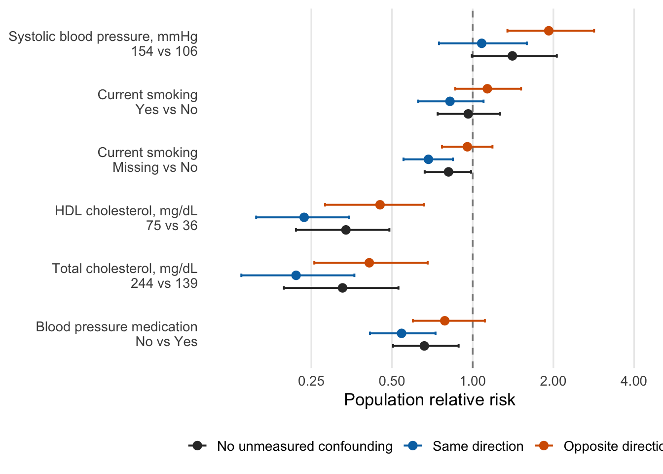
As in the primary analysis, \(Z\) denotes the common adjustment set, and \(\mu(x,z,u)\) is the outcome probability. BART estimates \(\eta_X(z)\) using probit BART for a categorical contrast and Gaussian BART for a continuous predictor. Probit BART estimates \(\eta_Y(x,z)\). The quantities \(\pi_U\), \(\beta_X\), and \(\beta_Y\) are fixed sensitivity parameters rather than estimated parameters. We fix the marginal prevalence at \(\pi_U=0.50\), following the default used in treatSens. A larger absolute value of either beta represents a stronger relationship between the unmeasured confounder and the corresponding observed variable; its sign determines the direction of that relationship.

For each target predictor, our target is its population relative risk (PRR). At each retained iteration, we predict the outcome under the two values defining that predictor’s contrast. The same sampled \(U\) is used under both interventions because \(U\) is a pre-exposure confounder. We then calculate the PRR using the same case-control population weights as in the primary analysis. An observation at a third category does not enter that contrast’s predictor model. Its predictor likelihood is therefore taken to be equal under \(U=0\) and \(U=1\) and supplies no information when \(U\) is updated. The observation still enters the outcome model and population PRR calculation. For example, Missing is neutral in the current-smoking Yes-versus-No predictor model, whereas Yes is neutral in the Missing-versus-No predictor model. In both analyses, all participants remain in the outcome analysis, and counterfactual prediction sets the original smoking variable to the two levels defining the requested contrast. We repeat the analysis for every contrast reported in the primary analysis, including both current-smoking contrasts.

We repeat this calculation over three \(\beta_X\) and \(\beta_Y\) scenarios: no unmeasured confounding, same-direction relationships with the predictor and outcome, and opposite-direction relationships. Each sensitivity chain begins from the corresponding chain in the reference outcome model. Predictors and sensitivity-parameter combinations are processed sequentially, while the eight chains within a combination run in parallel. We use 150 predictor-model burn-in iterations, 150 joint burn-in iterations, and 250 retained iterations per chain. We will increase these settings if the PRR or \(U\)-prevalence diagnostics indicate that longer chains are needed.

sensitivity_settings <- data.frame(
  beta_x = c(0, 0.5, 0.5),
  beta_y = c(0, 0.5, -0.5)
)

unmeasured_confounding_path <-
  "outputs/diagnostics/unmeasured_confounding/results.rds"

if (file.exists(unmeasured_confounding_path)) {
  unmeasured_confounding_sensitivity <-
    readRDS(unmeasured_confounding_path)
} else {
  unmeasured_confounding_sensitivity <- fit_all_proxy_sensitivity_models(
  analytic_df = analytic_df,
  y_var = final_config$outcome$name,
  config = final_config,
  predictor_stats_df = predictor_stats_df,
  sensitivity_settings = sensitivity_settings,
  reference_model = bart_fit,
  pi_u = 0.5,
  seed = 20260322L,
  x_burn = 150L,
  inner_burn = 150L,
  inner_keep = 250L,
  inner_thin = 1L
  )

  dir.create(
    "outputs/diagnostics/unmeasured_confounding",
    recursive = TRUE,
    showWarnings = FALSE
  )
  saveRDS(
    unmeasured_confounding_sensitivity,
    unmeasured_confounding_path
  )
  readr::write_csv(
    unmeasured_confounding_sensitivity$summary,
    "outputs/diagnostics/unmeasured_confounding/summary.csv"
  )
  readr::write_csv(
    unmeasured_confounding_sensitivity$diagnostics,
    "outputs/diagnostics/unmeasured_confounding/diagnostics.csv"
  )
}

The table reports the posterior PRR for each sensitivity-parameter combination. The \(\beta_X=0,\beta_Y=0\) row is the no-unmeasured-confounding benchmark. The remaining rows show how each PRR changes as the assumed relationships between \(U\), the focal predictor, and the outcome change.

unmeasured_confounding_sensitivity$summary |>
  knitr::kable(
    digits = 3,
    col.names = c(
      "Predictor",
      "Contrast",
      "$\\beta_X$",
      "$\\beta_Y$",
      "Posterior mean",
      "Posterior median",
      "2.5%",
      "97.5%"
    ),
    caption = "Population relative risks across unmeasured-confounding parameters"
  )

Population relative risks across unmeasured-confounding parameters
Predictor	Contrast	\(\beta_X\)	\(\beta_Y\)	Posterior mean	Posterior median	2.5%	97.5%
sbp	153.666666666667 vs 106.333333333333	0.0	0.0	1.436	1.406	0.993	2.060
sbp	153.666666666667 vs 106.333333333333	0.5	0.5	1.101	1.080	0.749	1.592
sbp	153.666666666667 vs 106.333333333333	0.5	-0.5	1.969	1.922	1.348	2.837
smoker_current	1 vs 0	0.0	0.0	0.972	0.962	0.740	1.265
smoker_current	1 vs 0	0.5	0.5	0.832	0.823	0.625	1.098
smoker_current	1 vs 0	0.5	-0.5	1.145	1.134	0.860	1.515
smoker_current	Missing vs 0	0.0	0.0	0.815	0.813	0.662	0.986
smoker_current	Missing vs 0	0.5	0.5	0.687	0.684	0.552	0.843
smoker_current	Missing vs 0	0.5	-0.5	0.959	0.955	0.768	1.185
hdl_c	75 vs 36	0.0	0.0	0.340	0.336	0.219	0.489
hdl_c	75 vs 36	0.5	0.5	0.239	0.235	0.156	0.345
hdl_c	75 vs 36	0.5	-0.5	0.454	0.451	0.281	0.658
tot_chol	244 vs 139	0.0	0.0	0.336	0.327	0.198	0.528
tot_chol	244 vs 139	0.5	0.5	0.229	0.219	0.137	0.362
tot_chol	244 vs 139	0.5	-0.5	0.425	0.411	0.256	0.679
bp_treated	0 vs 1	0.0	0.0	0.669	0.660	0.505	0.886
bp_treated	0 vs 1	0.5	0.5	0.551	0.543	0.414	0.727
bp_treated	0 vs 1	0.5	-0.5	0.806	0.787	0.598	1.110

The figure shows the same results graphically. Points are posterior medians and horizontal lines are 95% credible intervals. The dashed line marks a PRR of 1.

# Build and save the PRR sensitivity figure.
unmeasured_confounding_prr_plot <- plot_proxy_sensitivity_prrs(
  unmeasured_confounding_sensitivity$summary,
  final_config
)

ggplot2::ggsave(
  "outputs/diagnostics/unmeasured_confounding/prr_sensitivity.png",
  unmeasured_confounding_prr_plot,
  width = 9,
  height = 6.5,
  dpi = 600
)

unmeasured_confounding_prr_plot

The next table reports convergence diagnostics for the PRR and posterior prevalence of \(U\) within each predictor contrast and sensitivity setting.

unmeasured_confounding_sensitivity$diagnostics |>
  knitr::kable(
    digits = 2,
    col.names = c(
      "Predictor",
      "Contrast",
      "$\\beta_X$",
      "$\\beta_Y$",
      "Quantity",
      "R-hat",
      "Bulk ESS",
      "Tail ESS"
    ),
    caption = "Diagnostics for the unmeasured-confounding analysis"
  )

Diagnostics for the unmeasured-confounding analysis
Predictor	Contrast	\(\beta_X\)	\(\beta_Y\)	Quantity	R-hat	Bulk ESS	Tail ESS
sbp	153.666666666667 vs 106.333333333333	0.0	0.0	PRR	1.01	1118.53	1700.41
sbp	153.666666666667 vs 106.333333333333	0.0	0.0	U prevalence	NA	NA	NA
sbp	153.666666666667 vs 106.333333333333	0.5	0.5	PRR	1.01	1092.44	1709.99
sbp	153.666666666667 vs 106.333333333333	0.5	0.5	U prevalence	1.00	1687.07	1903.11
sbp	153.666666666667 vs 106.333333333333	0.5	-0.5	PRR	1.03	229.22	1044.11
sbp	153.666666666667 vs 106.333333333333	0.5	-0.5	U prevalence	1.00	1533.73	1653.15
smoker_current	1 vs 0	0.0	0.0	PRR	1.01	886.24	1660.80
smoker_current	1 vs 0	0.0	0.0	U prevalence	NA	NA	NA
smoker_current	1 vs 0	0.5	0.5	PRR	1.01	1228.88	1196.68
smoker_current	1 vs 0	0.5	0.5	U prevalence	1.00	1208.95	1735.30
smoker_current	1 vs 0	0.5	-0.5	PRR	1.01	984.48	1734.39
smoker_current	1 vs 0	0.5	-0.5	U prevalence	1.00	1381.62	1776.06
smoker_current	Missing vs 0	0.0	0.0	PRR	1.01	1092.63	1718.18
smoker_current	Missing vs 0	0.0	0.0	U prevalence	NA	NA	NA
smoker_current	Missing vs 0	0.5	0.5	PRR	1.01	1196.65	1792.48
smoker_current	Missing vs 0	0.5	0.5	U prevalence	1.00	970.10	1729.22
smoker_current	Missing vs 0	0.5	-0.5	PRR	1.01	1090.02	1566.88
smoker_current	Missing vs 0	0.5	-0.5	U prevalence	1.00	1055.84	1566.87
hdl_c	75 vs 36	0.0	0.0	PRR	1.07	90.62	560.53
hdl_c	75 vs 36	0.0	0.0	U prevalence	NA	NA	NA
hdl_c	75 vs 36	0.5	0.5	PRR	1.01	733.80	1564.83
hdl_c	75 vs 36	0.5	0.5	U prevalence	1.00	1674.62	1869.24
hdl_c	75 vs 36	0.5	-0.5	PRR	1.03	359.88	1094.18
hdl_c	75 vs 36	0.5	-0.5	U prevalence	1.00	1323.33	1750.31
tot_chol	244 vs 139	0.0	0.0	PRR	1.05	159.00	684.19
tot_chol	244 vs 139	0.0	0.0	U prevalence	NA	NA	NA
tot_chol	244 vs 139	0.5	0.5	PRR	1.07	91.35	626.47
tot_chol	244 vs 139	0.5	0.5	U prevalence	1.01	1668.13	1801.92
tot_chol	244 vs 139	0.5	-0.5	PRR	1.06	110.90	665.19
tot_chol	244 vs 139	0.5	-0.5	U prevalence	1.00	1594.73	1845.03
bp_treated	0 vs 1	0.0	0.0	PRR	1.01	1253.21	1747.60
bp_treated	0 vs 1	0.0	0.0	U prevalence	NA	NA	NA
bp_treated	0 vs 1	0.5	0.5	PRR	1.01	1479.81	1907.75
bp_treated	0 vs 1	0.5	0.5	U prevalence	1.01	924.06	1702.23
bp_treated	0 vs 1	0.5	-0.5	PRR	1.00	1321.64	1567.92
bp_treated	0 vs 1	0.5	-0.5	U prevalence	1.01	1011.37	1735.36